Exporting estimation tables
Laurent Bergé and Grant McDermott
2026-06-16
Source:vignettes/exporting_tables.Rmd
exporting_tables.RmdEstimating regression models, however handy and fast, is but one part
of the job. What we really care about is sharing our results with the
world, right? Alongside visualization, the canonical way to do this is
via regression tables. While R offers a variety of tabling software,
fixest provides its own dedicated tool—the function
etable—for viewing estimation tables in R and
exporting them to other formats like LaTeX.
The main advantage of etable over other options is its
native integration with the rest of the fixest ecosystem.
This makes it exceedingly easy to, for example, export multiple
estimation results with different types of standard-errors. It also
offers a lot of leeway for customization. Once you decided on your
preferred table aesthetic, you can even set default values to
permanently transform the style without modifying a further line of
code.
On the other hand, the two main etable limitations are
that only fixest objects can be exported, and the primary
output target is LaTeX (although the use of post-processing functions
opens up a lot of possibilities). We document some alternative tabling
options at the end of this document.
This article does not describe etable’s arguments in
detail (the help page provides many examples). Rather, it illustrates
some features that may be hidden at first sight.
Preliminaries
Throughout this document, we will primarily use data from the
airquality dataset. We also set a dictionary that will be used
to rename the variables used in etable. This dictionary is
set once and for all.
library(fixest)
data(airquality)

# Setting a dictionary
setFixest_dict(c(Ozone = "Ozone (ppb)", Solar.R = "Solar Radiation (Langleys)",
                 Wind = "Wind Speed (mph)", Temp = "Temperature"))
Displaying tables in the console
Let’s estimate the following four models and cluster the
standard-errors by Day:
# On multiple estimations: see the dedicated vignette
est = feols(Ozone ~ Solar.R + sw0(Wind + Temp) | csw(Month, Day),
            airquality, cluster = ~Day)
The default behaviour of etable is to return a
data.frame that prints nicely in your R console.1
etable(est)#> est.1 est.2 est.3
#> Dependent Var.: Ozone (ppb) Ozone (ppb) Ozone (ppb)
#>
#> Solar Radiation (Langleys) 0.115*** (0.023) 0.052* (0.020) 0.108** (0.033)
#> Wind Speed (mph) -3.11*** (0.799)
#> Temperature 1.88*** (0.367)
#> Fixed-Effects: ---------------- ---------------- ---------------
#> Month Yes Yes Yes
#> Day No No Yes
#> __________________________ ________________ ________________ _______________
#> S.E.: Clustered by: Day by: Day by: Day
#> Observations 111 111 109
#> R2 0.31974 0.63686 0.57983
#> Within R2 0.12245 0.53154 0.12074
#>
#> est.4
#> Dependent Var.: Ozone (ppb)
#>
#> Solar Radiation (Langleys) 0.051* (0.024)
#> Wind Speed (mph) -3.29*** (0.779)
#> Temperature 2.05*** (0.242)
#> Fixed-Effects: ----------------
#> Month Yes
#> Day Yes
#> __________________________ ________________
#> S.E.: Clustered by: Day
#> Observations 109
#> R2 0.81588
#> Within R2 0.61471
#> ---
#> Signif. codes: 0 '***' 0.001 '**' 0.01 '*' 0.05 '.' 0.1 ' ' 1What do we see? First, the variables are properly labeled. Second,
the fixed-effects section details which fixed-effects are included in
which model. Third, the type of standard-error is reported in a
dedicated row. Fourth, and perhaps most importantly for the
console-based etable output, the resulting table is
actually a standard R data.frame. This opens a lot of
possibility for further customization. Speaking of which…
It is possible to customize the look of our etable
console display using (a) the style.df argument and (b) the
postprocess.df argument, where the latter also allows you
to leverage tools from other packages. Let us consider each in turn.
Styling console output with style.df
You can change many elements of the data.frame with the
argument style.df whose input must come from the function
style.df. The style monitors many elements of the table, in
particular the titles of the sections. Let’s have an example:
etable(est, style.df = style.df(depvar.title = "", fixef.title = "",
                                fixef.suffix = " fixed effect", yesNo = "yes"))
#> est.1 est.2 est.3
#> Ozone (ppb) Ozone (ppb) Ozone (ppb)
#>
#> Solar Radiation (Langleys) 0.115*** (0.023) 0.052* (0.020) 0.108** (0.033)
#> Wind Speed (mph) -3.11*** (0.799)
#> Temperature 1.88*** (0.367)
#> Month fixed effect yes yes yes
#> Day fixed effect yes
#> __________________________ ________________ ________________ _______________
#> S.E.: Clustered by: Day by: Day by: Day
#> Observations 111 111 109
#> R2 0.31974 0.63686 0.57983
#> Within R2 0.12245 0.53154 0.12074
#>
#> est.4
#> Ozone (ppb)
#>
#> Solar Radiation (Langleys) 0.051* (0.024)
#> Wind Speed (mph) -3.29*** (0.779)
#> Temperature 2.05*** (0.242)
#> Month fixed effect yes
#> Day fixed effect yes
#> __________________________ ________________
#> S.E.: Clustered by: Day
#> Observations 109
#> R2 0.81588
#> Within R2 0.61471
#> ---
#> Signif. codes: 0 '***' 0.001 '**' 0.01 '*' 0.05 '.' 0.1 ' ' 1In the previous example, the dependent variable and fixed-effects
(FE) headers have been removed, and this is achieved with the (explicit)
arguments depvar.title and fixef.title.
Furthermore the suffix "fixed effect" is added to each
fixed-effect variable, and the indicator of which FE is included in
which model is slightly changed. There are more options that are
described in the style.df documentation.
Postprocessing with postprocess.df
Since the output of etable is a data.frame,
any formatting function handling data.frames can be
leveraged. It is then very easy to integrate it into
etable. Let’s have an example with the package
pander:
#>
#>
#> |                       |      est.1       |      est.2       |
#> |:--------------------------:|:----------------:|:----------------:|
#> |      Dependent Var.:       |   Ozone (ppb)    |   Ozone (ppb)    |
#> |                            |                  |                  |
#> | Solar Radiation (Langleys) | 0.115*** (0.023) |  0.052* (0.020)  |
#> |      Wind Speed (mph)      |                  | -3.11*** (0.799) |
#> |        Temperature         |                  | 1.88*** (0.367)  |
#> |       Fixed-Effects:       | ---------------- | ---------------- |
#> |           Month            |       Yes        |       Yes        |
#> |            Day             |        No        |        No        |
#> | __________________________ | ________________ | ________________ |
#> |      S.E.: Clustered       |     by: Day      |     by: Day      |
#> |        Observations        |       111        |       111        |
#> |             R2             |     0.31974      |     0.63686      |
#> |         Within R2          |     0.12245      |     0.53154      |
#>
#> Table: Table continues below
#>
#>
#>
#> |      est.3      |      est.4       |
#> |:---------------:|:----------------:|
#> |   Ozone (ppb)   |   Ozone (ppb)    |
#> |                 |                  |
#> | 0.108** (0.033) |  0.051* (0.024)  |
#> |                 | -3.29*** (0.779) |
#> |                 | 2.05*** (0.242)  |
#> | --------------- | ---------------- |
#> |       Yes       |       Yes        |
#> |       Yes       |       Yes        |
#> | _______________ | ________________ |
#> |     by: Day     |     by: Day      |
#> |       109       |       109        |
#> |     0.57983     |     0.81588      |
#> |     0.12074     |     0.61471      |
What did it do? First, it called the function
pandoc.table.return from within etable.
Second, the argument style is not from etable
but is from pander’s function. Indeed, all the arguments to
the postprocessing function are caught and passed to it. So far so good.
But you could say: why bother using the postprocessing function when we
could just use piping? You’re right, but wait a second for the next
section.
Setting default values
One important feature of etable is that you can set the
default values of almost all its arguments. This includes the
postprocessing function. Let’s change the default values of
style.df and postprocess.df:
my_style = style.df(depvar.title = "", fixef.title = "",
                    fixef.suffix = " fixed effect", yesNo = "yes")
setFixest_etable(style.df = my_style, postprocess.df = pandoc.table.return)
Since now pandoc.table.return is the default
postprocessing, all its arguments are added to
etable. So calls like that are valid even though
style or caption are not arguments
from etable:
etable(est[rhs = 2], style = "rmarkdown", caption = "New default values")#>
#>
#> | | est[rhs = 2].1 | est[rhs = 2].2 |
#> |:--------------------------:|:----------------:|:----------------:|
#> | | Ozone (ppb) | Ozone (ppb) |
#> | | | |
#> | Solar Radiation (Langleys) | 0.052* (0.020) | 0.051* (0.024) |
#> | Wind Speed (mph) | -3.11*** (0.799) | -3.29*** (0.779) |
#> | Temperature | 1.88*** (0.367) | 2.05*** (0.242) |
#> | Month fixed effect | yes | yes |
#> | Day fixed effect | | yes |
#> | __________________________ | ________________ | ________________ |
#> | S.E.: Clustered | by: Day | by: Day |
#> | Observations | 111 | 109 |
#> | R2 | 0.63686 | 0.81588 |
#> | Within R2 | 0.53154 | 0.61471 |Exporting tables to LaTeX
Displaying multiple estimations in the console is convenient for
interactive work. But most projects ultimately require us to export our
tables to a publishable format. For publishable research, that typically
means LaTeX. The good news is that etable has first-class
LaTeX support, which we demonstrate below.
Before continuing, let us first add a fifth estimation to the
previous example to show off some additional etable
functionality. This new estimation includes variables with varying
slopes:
est_slopes = feols(Ozone ~ Solar.R + Wind | Day + Month[Temp], airquality)Exporting this new estimation as LaTeX code simply requires the
argument tex = TRUE:
etable(est, est_slopes, tex = TRUE)#> \begingroup
#> \centering
#> \begin{tabular}{lccccc}
#> \tabularnewline \midrule \midrule
#> Dependent Variable: & \multicolumn{5}{c}{Ozone (ppb)}\\
#> Model: & (1) & (2) & (3) & (4) & (5)\\
#> \midrule
#> \emph{Variables}\\
#> Solar Radiation (Langleys) & 0.115$^{***}$ & 0.052$^{**}$ & 0.108$^{***}$ & 0.051$^{**}$ & 0.056$^{**}$\\
#> & (0.023) & (0.020) & (0.033) & (0.024) & (0.024)\\
#> Wind Speed (mph) & & -3.11$^{***}$ & & -3.29$^{***}$ & -3.05$^{***}$\\
#> & & (0.799) & & (0.779) & (0.678)\\
#> Temperature & & 1.88$^{***}$ & & 2.05$^{***}$ & \\
#> & & (0.367) & & (0.242) & \\
#> \midrule
#> \emph{Fixed-effects}\\
#> Month & Yes & Yes & Yes & Yes & Yes\\
#> Day & & & Yes & Yes & Yes\\
#> \midrule
#> \emph{Varying Slopes}\\
#> Temperature (Month) & & & & & Yes\\
#> \midrule
#> \emph{Fit statistics}\\
#> Observations & 111 & 111 & 109 & 109 & 109\\
#> R$^2$ & 0.31974 & 0.63686 & 0.57983 & 0.81588 & 0.82882\\
#> Within R$^2$ & 0.12245 & 0.53154 & 0.12074 & 0.61471 & 0.25843\\
#> \midrule \midrule
#> \multicolumn{6}{l}{\emph{Signif. Codes: ***: 0.01, **: 0.05, *: 0.1}}\\
#> \end{tabular}
#> \par\endgroupYou can copy and paste this output directly into your LaTeX editor.
But for most people, it will probably be more convenient (and safer) to
export the LaTeX table to disk as a named file that you can source from
your main article. We can do this by invoking the file
argument, which will automatically trigger tex = TRUE
too:
etable(est, est_slopes, file = "path/to/mytable.tex")Either way, you will end up with the following compiled table:
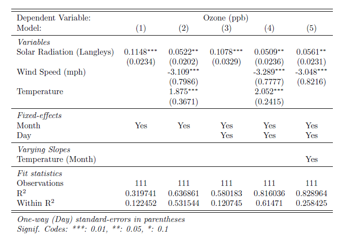
The default style of the table is rather dry. But just like the data
frame output, our LaTeX output is easily customized. We now illustrate
(a) how to change the look of the table with the argument
style.tex, and (b) how to include custom features with the
argument postprocess.tex.
Styling LaTeX output with style.tex
The argument style.tex defines how the table looks. It
allows an in-depth customization of the table. The table is split into
several components, each allowing some customization. The components of
a table and some of its associated keywords are described by the
following figure:
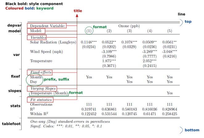
The argument style.tex only accepts outputs from the
function style.tex. That function is documented and
describes the different components that can be found in the previous
illustration.
The function style.tex has two starting points (in the
argument main), either the style of the first table
displayed, or a much more compact style named “aer”. Let’s show the same
table with the aer style, without stars beside the coefficients, and
different fit statistics:
etable(est, est_slopes, style.tex = style.tex("aer"),
       signif.code = NA, fitstat = ~ r2 + n, tex = TRUE)
Which yields the following table:

Postprocessing with postprocess.tex
When tex = TRUE, etable returns a character
vector. It is possible to modify it at will with the argument
postprocess.tex. When a postprocessing function is
detected, two additional tags are added to the character vector
identifying the start and end of the table ("%start:tab\\n"
and "%end:tab\\n").
If we want to set the rule widths of the table, we could write the following function:
set_rules = function(x, heavy, light){
  # x: the character vector returned by etable

  tex2add = ""
  if(!missing(heavy)){
    tex2add = paste0("\\setlength\\heavyrulewidth{", heavy, "}\n")
  }
  if(!missing(light)){
    tex2add = paste0(tex2add, "\\setlength\\lightrulewidth{", light, "}\n")
  }

  if(nchar(tex2add) > 0){
    x[x == "%start:tab\n"] = tex2add
  }

  x
}
Now we can summon that function from etable:
etable(est, est_slopes, postprocess.tex = set_rules, heavy = "0.14em", tex = TRUE)
Of course it is even more convenient to set set_rules as
the default postprocessing function, which provides a nice segue to the
next section.
Setting default values: LaTeX edition
To set the default values, like for the data.frame output, use
setFixest_etable:
setFixest_etable(style.tex = style.tex("aer", signif.code = NA), postprocess.tex = set_rules,
                 fitstat = ~ r2 + n)
Now we can access directly the arguments of the postprocessing function and the default style is the one of the second table:
etable(est, heavy = "0.14em", tex = TRUE)
Highlighting coefficients
Of course, LaTeX output gives you a lot more flexibility than
printing to the console. A sharp example of this is the ability to
highlight coefficients, which is especially useful for presentations.
etable offers three ways to highlight coefficients:
- using a frame,
- coloring the cells,
- giving a custom style to the coefficients.
The first two can be accessed via the highlight
argument. The last is implemented in the coef.style
argument.
Frame
By default, the highlight argument superimposes a frame
around the coefficients of interest. This is done thanks to some
tikz magic found in tex
stack exchange.
The syntax is "options" = "coefficients location". The
coefficient location can be expressed in several ways:
- the coefficient name: the full row is selected. Ex:
Petal.Lwill select thePetal.Lengthrow. - the coefficient name followed by
@and column ranges: in the coefficient row, only selects the given columns. Ex:Petal.L@1,3-4will select, in the rowPetal.Length, the columns 1, 3 and 4. - a vector of two coefficient cells: selects the full range from
top-left to bottom right. Ex:
c("Petal.L@2", "Petal.W@3")will select a range from the second column ofPetal.Lengthto the third column ofPetal.Width.
Let’s have an example illustrating the three ways to select the
coefficients and some options. We switch to the iris
dataset here since its Species factor gives us a nice
split-sample layout. We also increase the row heights with
arraystretch to facilitate the highlighting:
nm = names(iris)
est_iris = feols(.[nm[1]] ~ .[nm[2:4]], iris, fsplit = ~Species)

etable(est_iris, arraystretch = 1.5, tex = TRUE,
       highlight = .("Sepal@1",
                     "cyan4, square" = "Petal.L@3-4",
                     "thick5, sep8, darkgreen!90, se" = "Petal.W"))
There are five main options:
-
se: whether the standard-error should be included, -
sep0tosep9: the separation between the coefficients and the frame (default issep3), -
thick1tothick6: the thickness of the line of the frame (default isthick6), -
square: whether the frame box should have square corners, -
color!alpha: an R color followed by an (optional) alpha value. It is important to emphasize that it should be a valid R color (not LaTeX). The color is then translated into LaTeX and is guaranteed to work. The error handling is done in R to avoid problems appearing at the LaTeX compilation time which would be hard to debug.
Row colors
Instead of highlighting coefficients with a frame, row color
highlighting can be used. It is monitored with the same argument
highlight and in fact you only have to add the option
rowcol to make it work. Let’s replicate the previous
example with row color:
etable(est_iris, arraystretch = 1.5, tex = TRUE,
       highlight = .(rowcol = "Sepal@1",
                     "rowcol, cyan4!70" = "Petal.L@3-4",
                     "rowcol, darkgreen!40, se" = "Petal.W"))
As opposed to the previous example, we only have increased the
transparency of the colors with the color!alpha syntax.
Contrary to the frame, there are no options for the row coloring
apart from the color itself and se to include the
standard-errors.
Style
Using the same syntax as before to select the coefficients,
it is possible to completely customize the coefficient cells. The syntax
is coef.style = .("style" = "coefficients location") with
style equal to LaTeX code containing the tag :coef: which
will be replaced with the coefficient value. Alternatively, using the
tag :coef_se: will apply the style both to the coefficient
and the standard-error.
Here is the replication of the previous example with another highlighting:
etable(est_iris, tex = TRUE,
       coef.style = .(":coef:$\\bigstar$" = "Sepal@1",
                      "**:coef:**" = "Petal.L@3-4",
                      "\\color{BrickRed} :coef_se:" = "Petal.W"))
LaTeX extras
While style.tex, postprocess.tex,
highlight and co. can get you pretty far, it’s possible to
customize to your etable output even further with the help
of some third-party LaTeX packages. Note that you’ll have to install
these these third-party packages yourself, but the etable
code will execute regardless. Let’s see some examples.
threeparttable
The threeparttable LaTeX package lets you attach notes
that automatically match the table width. You can enable it via
style.tex(), and access notes from the global dictionary to
avoid repetitions:
# First define notes in the dictionary
setFixest_dict(c(note1 = paste0("*Notes*: This is a note that illustrates how to access notes ",
                                "from the dictionary."),
                 source = "*Sources*: Somewhere from the net."))

etable(est,
       style.tex = style.tex("aer", tpt = TRUE, notes.tpt.intro = "\\footnotesize"),
       notes = c("note1", "source"), tex = TRUE)
The table notes are adjusted to the table width thanks to
threeparttable and the notes are accessed directly with
their keys. The argument notes.tpt.intro inserts LaTeX code
right before the first \\item of threeparttable: in this
case, it sets the font to footnotesize.
In general, it is advised to set the value of tpt and
the notes.tpt.intro globally. Then if one wants to change
the value of notes.tpt.intro, instead of typing
style.tex = style.tex(notes.tpt.intro = "stuff"), the first
element of notes will replace notes.tpt.intro
if it starts with an "@":
# Setting up tpt globally
my_style = style.tex(tpt = TRUE,
                     notes.tpt.intro = "\\footnotesize")
setFixest_etable(style.tex = my_style)

# Below is identical to:
#  etable(est,
#         style.tex = style.tex(notes.tpt.intro = "\\Large"),
#         notes = "These notes are large.")
etable(est, notes = c("@\\Large", "These notes are large."), tex = TRUE)
adjustbox
The adjustbox LaTeX package can resize a table to fit a
target width—especially useful for wide tables that would otherwise
overflow.
By default if adjustbox = TRUE, the table is nested in
an adjustbox environment with the options
width = 1\\textwidth, center. This argument can be equal to
a number, in which case it will be treated as the desired text width.
Otherwise it accepts any character string.
Let’s have an example with a large table that would otherwise overflow:
est_many = feols(Ozone ~ mvsw(Solar.R, Wind, Temp), airquality)
etable(est_many, adjustbox = 1.1, tex = TRUE)
makecell
fixest supports markdown markup (*,
**, ***) for italics, bold, and bold-italics
in most user-added text. It also supports the makecell
LaTeX package for multi-line cells: simply include "\n" in
your text. Here’s an example:
# Reset defaults from previous sections
setFixest_etable(reset = TRUE)
etable(est, headers = .("\n\n Short header" = 2, "*Very* \n **long** \n ***header***" = 2),
       tex = TRUE)
Exporting tables to other formats
The primary output targets for etable are regular R data
frames and LaTeX. This still leaves a variety of other formats off the
table, including .html, .docx and
.typ. While we don’t offer “native” support for these
formats—and users may consider alternative software if that suits
their workflow—we do at least provide a workaround that covers most
other cases. Specifically, we can export etable
objects as PNGs, which then allows for easy inclusion in HTML,
MS Word documents, etc. We explain how this works below, but please note
that it requires the following software to be installed first:
-
pdflatex(shipped in most LaTeX distributions) or the R packagetinytex, -
imagemagick and ghostscript, or
the R package
pdftools.
Exporting tables as PNGs
(Our thanks to Avishay-Rizi for the initial suggestion that led to this feature.)
The workaround here can be summarized as
etable -> LaTeX -> PDF -> PNG. First, we take our
etable call and compile a standalone LaTeX document
(containing only the table) to PDF. Then, we call
imagemagick under the hood to convert the PDF into a PNG
file.
While this workflow might seem a bit convoluted, we do our best to
automate the process so that everything “just works” from the end user’s
perspective. In particular, we cover the most common use cases via
convenience arguments for Quarto and Rmarkdown output
(markdown) and integrated IDE viewer
(view).
Quarto and Rmarkdown: argument markdown
This option works only within Quarto and
Rmarkdown documents and is ignored otherwise. If
markdown = TRUE the output becomes always a LaTeX table,
even when tex = FALSE (default). The output within the
rendered document is contingent on the type of target file. If the
document is being rendered to PDF, then a regular LaTeX table is
returned. However, if the document is not being rendered to PDF
(especially if it is an HTML file), then:
- the PNG of the table is generated and saved in
images/etable/, so that successive calls don’t need to re-generate the PNGs (i.e. this is caching), - the generated image is inserted in the document in an
<img>tag, - that
<img>tag is inserted in a<div>container of classetable.
This ensures that the tables are the same whether the output is a PDF
or an HTML document. Since the table is embedded in a
<div> container, you can add custom CSS to further
customize how it looks (see the CSS section
below).
Fun fact: all of the rendered tables from the postprocessing section
onward in this article were generated using
markdown = TRUE!
CSS for custom HTML output
When using markdown = TRUE, the image of the table is
embedded in a <div> container whose default class is
etable. You can set the class of that
<div> manually with the argument
div.class and apply custom CSS styling. You can add this as
a custom CSS entry to your Quarto/Rmarkdown document for exporting to
HTML, or bundle it as part of a theme. An example of the latter can be
found in the clean
theme for Quarto Reveal.js format.
Monitoring the look of the tables: the argument page.width
As mentioned, to generate a PNG image, a LaTex table is first embedded in a standalone LaTeX document, then the document is compiled to generate a PDF, and the PDF is converted to PNG. The default LaTex document has no page size and no margin, meaning that whatever the width of the table (be it two or twenty columns), it will always take 100% of the width of the PDF.
While this property is fine when displaying on the viewer, it makes
the tables look odd and inconsistent in an HTML document. The
page.width argument sets the width and side margins of the
page in which the table will be inserted. The goal is to mimic the
placement of the table in a real PDF document (i.e. in your
article). For instance, page.width = "a4" will set an A4
page width and 2cm side margins on both sides. This argument can be
customized at will: e.g. 8.5in, 1.1in will lead to a page
width of 8.5 inches with 1.1 inch side margins (the only constraint is
that the unit of the width should be the same as the unit of the
margin).
When page.width is set up, all tables in an HTML
document will be consistent: the font will be the same across tables. On
top of that, it also enables a couple of specific features. First, if
the table is too narrow, you can use a tabularx table (with the
argument tabular) and the table will be as large as the
“text” width. Second, if the table overflows, you can adjust it with the
argument adjustbox to make it fit the text width.
RStudio and Positron (VS Code): argument view
The most popular R IDEs like RStudio and Positron (VS Code) come with
their own dedicated viewer panels. If you would like to display the
results of a regression table in one of these viewers, simply use the
etable(..., view = TRUE) argument. This will invoke the PNG trick that we described above
and display the resulting table snapshot in your IDE’s viewer.
Note that it can be useful to cache the PNG outputs to avoid the
compilation run-time; at least if you plan on displaying the same tables
multiple times in a row. Caching can be enabled with
setFixest_etable(view.cache = TRUE). The images are then
saved in a temporary directory that the algorithm tries to find even
across sessions (i.e., it should enable long-term caching).
Custom fit statistics
It is often useful to include in a table some fit statistics that are
not standard, or simply that may not be included in fixest
built-in fit statistics. While it is possible to include any extra line
in the table with the argument extralines, this is rather
cumbersome and possibly error-prone if this task has to be repeated.
To avoid that kind of issue, fixest allows the user to
register custom fit statistics. Once they are registered, they can be
seamlessly called via the fitstat argument in
etable.
Let’s continue with the previous example using the
airquality data set, and now let’s display different
p-values of statistical significance for the variable
Solar.R. These p-values will vary depending on how we
compute the VCOV matrix.
Here is an example that will shortly be explained:
# Reset defaults from previous sections
setFixest_etable(reset = TRUE)
setFixest_dict(c(Ozone = "Ozone (ppb)", Solar.R = "Solar Radiation (Langleys)",
                 Wind = "Wind Speed (mph)", Temp = "Temperature"))

fitstat_register(type = "p_s", alias = "pvalue (standard)",
                 fun = function(x) pvalue(x, vcov = "iid")["Solar.R"])

fitstat_register(type = "p_h", alias = "pvalue (Heterosk.)",
                 fun = function(x) pvalue(x, vcov = "hetero")["Solar.R"])

fitstat_register(type = "p_day", alias = "pvalue (Day)",
                 fun = function(x) pvalue(x, vcov = ~Day)["Solar.R"])

fitstat_register(type = "p_month", alias = "pvalue (Month)",
                 fun = function(x) pvalue(x, vcov = ~Month)["Solar.R"])

# Now we display the results with the new fit statistics
etable(est, fitstat = ~ . + p_s + p_h + p_day + p_month)
#> est.1 est.2
#> Dependent Var.: Ozone (ppb) Ozone (ppb)
#>
#> Solar Radiation (Langleys) 0.1148*** (0.0234) 0.0522* (0.0202)
#> Wind Speed (mph) -3.109*** (0.7986)
#> Temperature 1.875*** (0.3671)
#> Fixed-Effects: ------------------ ------------------
#> Month Yes Yes
#> Day No No
#> __________________________ __________________ __________________
#> S.E.: Clustered by: Day by: Day
#> Observations 111 111
#> R2 0.31974 0.63686
#> Within R2 0.12245 0.53154
#> pvalue (standard) 0.00022 0.02957
#> pvalue (Heterosk.) 6.64e-6 0.02268
#> pvalue (Day) 3e-5 0.01468
#> pvalue (Month) 0.06066 0.26992
#>
#> est.3 est.4
#> Dependent Var.: Ozone (ppb) Ozone (ppb)
#>
#> Solar Radiation (Langleys) 0.1078** (0.0329) 0.0509* (0.0236)
#> Wind Speed (mph) -3.289*** (0.7791)
#> Temperature 2.052*** (0.2420)
#> Fixed-Effects: ----------------- ------------------
#> Month Yes Yes
#> Day Yes Yes
#> __________________________ _________________ __________________
#> S.E.: Clustered by: Day by: Day
#> Observations 109 109
#> R2 0.57983 0.81588
#> Within R2 0.12074 0.61471
#> pvalue (standard) 0.00196 0.03720
#> pvalue (Heterosk.) 0.00093 0.02679
#> pvalue (Day) 0.00282 0.03973
#> pvalue (Month) 0.02600 0.29584
#> ---
#> Signif. codes: 0 '***' 0.001 '**' 0.01 '*' 0.05 '.' 0.1 ' ' 1The function fitstat_register is a tool to add fit
statistics in the fitstat engine. The first argument,
type, is the code name by which the statistic is to be
summoned. The argument alias provides the row name of the
statistics: how it should look in the table. Finally in the
fun argument is the function computing the statistic. That
function must apply to a fixest estimation and must also
return a single value.
Once these statistics are registered, they can seamlessly be summoned
with the argument fitstat and will appear in the order the
user provides. Note that the dot in
fitstat = ~ . + p_s + etc represents the default statistics
to be displayed and need not be there.
Other tabling software
Thanks to community contributors, fixest objects are
supported by both broom and parameters. These two
packages provide the common building blocks for extracting relevant
information from a huge variety of R model classes, which in turn opens
the possibility for easy integration with generic tabling software.
Two of the most popular tabling packages in R are modelsummary
and gtsummary,
which are both excellent and happily recommended. You may well prefer to
use either of these if you are working with additional model classes
beyond fixest objects, or you require the seamless
integration that they provide for different Quarto and Rmarkdown output
formats (including HTML, MS Word, and Typst). The downside to using
these external packages is that they are, necessarily, less tightly
integrated with fixest objects and may require more code to
achieve the same results.
Regardless of your preferences, here are some tips for working with
fixest objects and alternative tabling software.
Multiple estimations, like the object
estin the previous examples, are a bit special andbroommethods can’t apply directly. To export them, you first need to coerce the results into a list: by simply usingas.list(est).-
By default, in
fixestthe estimations are separated from the calculation of the VCOV matrices. That’s not a problem when usingetablesince, after providing the argumentvcovorcluster, all VCOVs are calculated at once. Using other tools for exportation requires a call tosummaryfor each model to compute the appropriate standard-errors. But this process can also be automatized. The function.l()can be used to coerce severalfixestobjects to whichsummarycan then be applied, for example:The previous code returns a list of the five estimations for which the standard-errors are all clustered at the Month level, and can then be exported with external software.