On Standard Errors

This vignette discusses how the fixest package computes the standard-errors of coefficients obtained from (generalized) linear regressions (i.e. from feols, feglm/fepois). Please note that here we don’t discuss much the why, but mostly the how. For an introduction to the topic, see the paper by Zeileis, Koll and Graham (2020).

The first part of this vignette describes the main ways standard-errors can be computed in fixest’s estimations.

The second part discusses the nitty-gritty details about the possible choices surrounding small sample correction.

The third part illustrates how to replicate standard-errors obtained from estimation methods of other software.

Review of theory

The regression coefficient takes the form $\hat{\beta} \equiv \left( X' X \right)^{-1} X' y,$ where $X$ is the $n \times K$ matrix of predictor variables for the sample and $y$ is the $n \times 1$ vector of the outcome variable. Plugging in the working model for $y$ , yields

$\hat{\beta} \equiv \left( X' X \right)^{-1} X' \left( X \beta_0 + \varepsilon \right),$ where $\beta_0$ corresponds to the population regression coefficent and $\varepsilon$ is the $n \times 1$ vector of prediction errors.

This yields: $\hat{\beta} - \beta_0 = \left( X' X \right)^{-1} X' \varepsilon.$

This immediately suggests the standard asymptotic distribution $\hat{\beta} \sim \mathcal{N} \left( \beta_0, \left( X' X \right)^{-1} X' \Sigma X \left( X' X \right)^{-1} \right),$ where $\Sigma = \mathbb{E} \left[ \varepsilon \varepsilon' \right]$ is the covariance matrix of the error term. The matrix $\left( X' X \right)^{-1} X' \Sigma X \left( X' X \right)^{-1}$ is often called the “sandwich” form inspiring the name of the classic R package, sandwich. Continuing with the name, $\left( X' X \right)^{-1}$ show up on each side and are called the “bread”. The bread is immediately estimated from the data. The “meat”, $X' \Sigma X$ , on the other hand is the source of all the difficulties, since we do not observe the prediction error $\varepsilon$ directly.

The matrix $\Sigma$ takes the form: $\Sigma = \begin{bmatrix} \sigma_1^2 & \sigma_{1, 2} & \dots & \sigma{1, n} \\ \sigma_{2, 1} & \sigma_{2}^2 & \dots & \sigma{2, n} \\ \vdots & \vdots & \ddots & \vdots \\ \sigma_{n, 1} & \sigma_{n, 2} & \dots & \sigma_{n}^2 \\ \end{bmatrix}.$ The elements $\sigma_{i,j}$ denote the covariance between unit $i$ and unit $j$ ’s error term: $\mathbb{E}[\varepsilon_i \varepsilon_j]$ .

A few common cases:

“Non-correlated”: If we think the error terms are non-correlated across observations, then σi,j=0\sigma_{i,j} = 0 when i≠ji \neq j and Σ\Sigma is a diagonal matrix.
- If $\sigma_i^2 = \sigma^2$ , this is called homoskedastic errors.
- If $\sigma_i^2$ is allowed to vary, this is called heteroskedastic errors.
“Clustering”: If we think units belong to distinct clusters where errors can be correlated, i.e. σi,j=0\sigma_{i,j} = 0 when c(i)≠c(j)c(i) \neq c(j) then Σ\Sigma is block-diagonal
- If we think there are multiple clusters, then we can use “multi-way clustering”
“Autocorrelated”: We might think observations “close together” have covariance, but that covariance decays with distance
- “temporally autocorrelated”: if distance is measured over time for a given unit (panel or time-series)
- “spatially correlated”: if distance is measured over space

There is no general answer to which setting you might be in; hence all the discussion on “how do you cluster your standard errors” or “what standard errors are you showing”. However, in general, we estimate standard errors by plugging in $\hat{\Sigma}$ into the sandwich form above. To estimate $\hat{\Sigma}$ , we use our regression residuals, $\hat{\varepsilon}$ : $\hat{\Sigma}_{i, j} = w_{i, j} \hat{\varepsilon}_i \hat{\varepsilon}_j,$ where $w_{i,j}$ is a weight term (depending on the choice of vcov estimator). For example, if we are using “HC1” standard errors, then $w_{i,i} = 1$ and $w_{i,j} = 0$ whenever $i \neq j$ . For clustered standard errors, we use: $w_{i, j} = 1 / N_{c(i)}$ whenever $c(i) = c(j)$ and $w_{i,j} = 0$ otherwise.

Since we use $\hat{\varepsilon}_i$ instead of the true $\varepsilon_i$ , it turns out that our standard error estimates will typically be too small. This problem is that the residuals tend to be “too small” because they are in-sample prediction errors (regressions overfit the sample). This problem is particularly large when the sample size is too “small”. Usually, we apply a “small-sample correction” to make the standard errors slightly larger. These corrections are usually “ad hoc” and can vary from package to package. For this reason, we delay discussion to the end of the vignette (hic sunt leones).

FWL for variance-covariance matrix

The Frisch-Waugh-Lovell theorem is central to the fixest package: we can first residualize fixed-effects from the matrix of predictors and then run a much simpler regression of $\tilde{y}$ on $\tilde{X}$ (with $\tilde{\cdot}$ representing the fixed-effect residualizing. What does this due to our estimation of the fixed-effects?

Peng Ding shows that the standard Frisch-Waugh-Lovell logic applies to estimation of the variance-covariance matrix of regression coefficients (in most cases). That is, we can use $\left( \tilde{X}' \tilde{X} \right)^{-1} \tilde{X}' \hat{\Sigma} \tilde{X} \left( \tilde{X}' \tilde{X} \right)^{-1}.$ As long as we remember to update our degrees of freedom correction to account for the fixed-effects, our estimates will be identical to the “full regression”. Therefore, fixest is able to maintain its very fast estimation approach when estimating standard errors.¹

Generalized linear models

For generalized linear models, a similar sandwich form arrives. In fixest, the coefficients are estimated via a “iterative weighted least squares” procedure. Therefore, we get a similar formula as before: $\hat{V}(\hat{\beta}) = (X' W X)^{-1} (X' \Sigma X) (X' W X)^{-1},$ where $W$ is a diagonal $n \times n$ matrix of “working weights”. Again, all the action comes into the matrix $\Sigma$ .² Therefore, the exact same intuition from above can be used: select the choice of vcov based on how you think error terms might be correlated to one another.

How standard-errors are computed in `fixest`

There are two components defining the standard-errors in fixest. The main type of standard-error is given by the argument vcov, the small sample correction is defined by the argument ssc.

The argument `vcov`

There are three main ways to specify the VCOV using the argument vcov: 1) with a character string, 2) with a formula, 3) with a vcov_* function. When a character string, the argument vcov can be equal to either: "iid", "hetero"/"HC1", "HC2", "HC3", "cluster", "twoway", "NW", "DK", or "conley".

Classical standard errors

For classical standard errors, set vcov = "iid". This assumes that $\sigma_i^2 = \sigma^2$ , i.e. the errors are non-correlated and homoskedastic. This is the default primarily for speed of estimation, but in practice it is never recommended as homoskedasticity is not likely to hold.

Heteroskedasticity-robust standard errors

There are a few options for heteroskedasticity-robust standard errors, named HC1, HC2, and HC3. They all allow $\sigma_i^2$ to vary by $i$ , but assumes non correlated errors across $i, j$ . The HC1 estimator (White 1980) is the fastest to calculate and works well with “large samples”. This can be used with vcov = "HC1" or vcov = "hetero".

However, HC1 performs poorly for small samples. HC2 and HC3 work well in small samples, but can be quite costly to compute with large samples. These can be used with vcov = "HC2" and vcov = "HC3". See James MacKinnon’s review article for a more detailed discussion.

Cluster-robust standard errors

Cluster robust standard errors allow for correlation within a cluster (or multiple clusters). This can be used by passing a one-sided formula, vcov = ~ clust_var, to specify the clustering variable. If vcov = "cluster" is used, fixest will use the first fixed-effect variable as the clustering variable (though it is often better to be explicit).

For multi-way clustering (e.g. clustering a panel of students to be clustered by class and over time) can be done with vcov = ~ clust1 + clust2. Similarly, vcov = "twoway" will automatically use the first two fixed-effect variables. Cameron and Miller (2015) write a practical guide to clustering that discusses this in more detail.

Inference with a small number of clusters can be potentially problematic for classic clustering methods. The intuition the “large N” we need for asymptotics to approximate the sample distribution well is the number of groups $G$ . One solution to this is to use a small-sample correction and a $t$ -distribution, but this can perform poorly if $G$ is very small. MacKinnon and Webb (2020) provide more detailed guidance on what to do in this case.

Abadie, Athey, Imbens, and Wooldridge (2023) provide a more detailed discussion of whether clustering is needed in causal inference methods.

Heteroskedasticity and auto-corrleation robust standard errors

In the context of time series, vcov = "NW" (Newey and West (1987)) account for temporal correlation between the errors. For panel data, vcov = "DK" (Driscoll and Kraay (1998)) account for temporal correlation between the errors. The two differing on how to account for heterogeneity between units. Their implementation is based on Millo (2017).

In either case, the asymptotic framework requires the number of time-periods, $T$ , to be large (regardless of the number of units in the panel context). If you have panel data but small $T$ , clustering at the unit-level is preferabble. The value of $T$ will be relevant in small-sample corrections, discussed below.

Spatial-correlation robust standard errors

Finally, vcov = "conley" accounts for spatial correlation of the errors based on Conley (1999). To account for spatial correlation, fixest needs to know the “x” and “y” coordinates. fixest tries to be smart and look for these in the dataset by column names, but if this fails, you need to use vcov = vcov_conley(lat = "xname", lon = "yname").

Other options

fixest was designed with flexibility in mind. It is possible to use other methods for estimation via the vcov argument. In this setting, a variance-covariance matrix can be “attached” to a fixest object using the summary function and this matrix will be used for post-estimation commands. For example, we can estimate bootstrapped standard errors via sandwich::vcovBS or we could write a custom function that works with a fixest object.

library(fixest)
est = feols(mpg ~ wt + hp, mtcars)

## Simple function that computes a Bayesian bootstrap
vcov_bboot = function(x, n_sim = 100) {
  core_env = update(x, only.coef = TRUE, only.env = TRUE)
  n_obs = x$nobs

  res_all = vector("list", n_sim)
  for (i in 1:n_sim) {
    # est_env updates estimate using new weights
    res_all[[i]] = est_env(env = core_env, weights = rexp(n_obs, rate = 1))
  }

  res = do.call(rbind, res_all)

  # Could return just `var(res)` but the named list will display a nice name in `etable`
  return(list("Bayesian Bootstrap" = var(res)))
}

set.seed(1)
est_bboot_se = summary(est, vcov = vcov_bboot(est))
etable(est, est_bboot_se)

#>                                est        est_bboot_se
#> Dependent Var.:                mpg                 mpg
#>                                                       
#> Constant          37.23*** (1.599)    37.23*** (1.946)
#> wt              -3.878*** (0.6327)  -3.878*** (0.6159)
#> hp              -0.0318** (0.0090) -0.0318*** (0.0061)
#> _______________ __________________ ___________________
#> S.E. type                      IID  Bayesian Bootstrap
#> Observations                    32                  32
#> R2                         0.82679             0.82679
#> Adj. R2                    0.81484             0.81484
#> ---
#> Signif. codes: 0 '***' 0.001 '**' 0.01 '*' 0.05 '.' 0.1 ' ' 1

Small sample correction

As discussed above, plugging in residuals from a regression to estimate the variance of the true error term will create standard error estimates that are too small. The small sample correction aims to “correct” this problem by increasing the estimate $\tilde{V}$ by some factor that is $\geq 1$ and approaches $1$ as the sample gets larger. These corrections only make a meaninful adjustment when the sample is small (or the number of clusters is small), hence the name.

The type of small sample correction applied is defined by the argument ssc which accepts only objects produced by the function ssc. The main arguments of this function are K.adj, K.fixef and G.adj. Each of them is detailed below.

Before we dive into the details, here is an example of modifying the small sample correction:

data(trade)
gravity = feols(
  log(Euros) ~ log(dist_km) | Destination + Origin + Product + Year,
  trade
)
# Two-way clustered SEs
summary(gravity, vcov = "twoway")

#> OLS estimation, Dep. Var.: log(Euros)
#> Observations: 38,325
#> Fixed-effects: Destination: 15,  Origin: 15,  Product: 20,  Year: 10
#> Standard-errors: Clustered (Destination & Origin) 
#>              Estimate Std. Error  t value   Pr(>|t|)    
#> log(dist_km) -2.16988   0.171367 -12.6621 4.6802e-09 ***
#> ---
#> Signif. codes:  0 '***' 0.001 '**' 0.01 '*' 0.05 '.' 0.1 ' ' 1
#> RMSE: 1.74337     Adj. R2: 0.705139
#>                 Within R2: 0.219322

# Two-way clustered SEs, without small sample correction
summary(gravity, vcov = "twoway", ssc = ssc(K.adj = FALSE, G.adj = FALSE))

#> OLS estimation, Dep. Var.: log(Euros)
#> Observations: 38,325
#> Fixed-effects: Destination: 15,  Origin: 15,  Product: 20,  Year: 10
#> Standard-errors: Clustered (Destination & Origin) 
#>              Estimate Std. Error  t value   Pr(>|t|)    
#> log(dist_km) -2.16988   0.165494 -13.1115 2.9764e-09 ***
#> ---
#> Signif. codes:  0 '***' 0.001 '**' 0.01 '*' 0.05 '.' 0.1 ' ' 1
#> RMSE: 1.74337     Adj. R2: 0.705139
#>                 Within R2: 0.219322

Say you have $\tilde{V}$ the variance-covariance matrix (henceforth VCOV) before any small sample adjustment. Argument K.adj can be equal to TRUE or FALSE, leading to the following adjustment:

When the estimation contains fixed-effects, the value of $K$ in the previous adjustment can be determined in different ways, governed by the argument K.fixef. To illustrate how $K$ is computed, let’s use an example with individual (variable id) and time fixed-effect and with clustered standard-errors. The structure of the 10 observations data is:

The standard-errors are clustered with respect to the cluster variable, further we can see that the variable id is nested within the cluster variable (i.e. each value of id “belongs” to only one value of cluster; e.g. id could represent US counties and cluster US states).

The argument K.fixef can be equal to either "none", "nonnested" or "full". Then $K$ will be computed as follows:

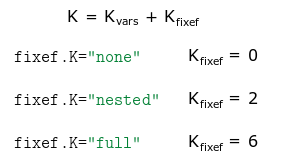
Where $K_{vars}$ is the number of estimated coefficients associated to the variables. K.fixef="none" discards all fixed-effects coefficients. K.fixef="nonnested" discards all coefficients that are nested (here the 5 coefficients from id). Finally K.fixef="full" accounts for all fixed-effects coefficients (here 6: equal to 5 from id, plus 2 from time, minus one used as a reference [otherwise collinearity arise]). Note that if K.fixef="nonnested" and the standard-errors are not clustered, this is equivalent to using K.fixef="full".

The last argument of ssc is G.adj. This argument is only relevant when the standard-errors are clustered or when they are corrected for serial correlation (Newey-West or Driscoll-Kraay). Let $M$ be the sandwich estimator of the VCOV without adjustment. Then for one-way clustered standard errors:

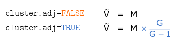
With $G$ the number of unique elements of the cluster variable (in the previous example $G=2$ for cluster).

The effect of the adjustment for two-way clustered standard-errors is as follows:

Using the data from the previous example, here the standard-errors are clustered by id and time, leading to $G_{id}=5$ , $G_{time}=2$ , and $G_{id,time}=10$ .

When standard-errors are corrected for serial correlation, the corresponding adjustment applied is $G_{time} / (G_{time} - 1)$ .

Yet more details

We now detail three more elements: K.exact, G.df and t.df.

Argument K.exact is only relevant when there are two or more fixed-effects. By default all the fixed-effects coefficients are accounted for when computing the degrees of freedom. In general this is fine, but in some situations it may overestimate the number of estimated coefficients. Why? Because some of the fixed-effects may be collinear, the effective number of coefficients being lower. Let’s illustrate that with an example. Consider the following set of fixed-effects:

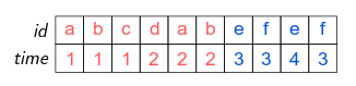
There are 6 different values of id and 4 different values of time. By default, 9 coefficients are used to compute the degrees of freedom (6 plus 4 minus one reference). But we can see here that the “effective” number of coefficients is equal to 8: two coefficients should be removed to avoid collinearity issues (any one from each color set). If you use K.exact=TRUE, then the function fixef is first run to determine the number of free coefficients in the fixed-effects, this number is then used to compute the degree of freedom.

Argument G.df is only relevant when you apply two-way clustering (or higher). It can have two values: either "conventional", or "min" (the default). This affects the adjustments for each clustered matrix. The "conventional" way to make the adjustment has already been described in the previous equation. If G.df="min" (again, the default), and for two-way clustered standard errors, the adjustment becomes:

Now instead of having a specific adjustment for each matrix, there is only one adjustment of $G_{min}/(G_{min}-1)$ where $G_{min}$ is the minimum cluster size (here $G_{min}=\min(G_{id},G_{time})$ ).

Argument t.df is only relevant when standard-errors are clustered. It affects the way the p-value and confidence intervals are computed. It can be equal to: either "conventional", or "min" (the default). By default, when standard-errors are clustered, the degrees of freedom used in the Student t distribution is equal to the minimum cluster size (among all clusters used to cluster the VCOV) minus one. If t.df="conventional", the degrees of freedom used to find the p-value from the Student t distribution is equal to the number of observations minus the number of estimated coefficients.

Replicating standard-errors from other methods

This section illustrates how the results from fixest compares with the ones from other methods. It also shows how to replicate the latter from fixest.

The data set and heteroskedasticity-robust SEs

Using the Grunfeld data set from the plm package, here are some comparisons when the estimation doesn’t contain fixed-effects.

library(sandwich)
library(plm)

data(Grunfeld)

# Estimations
res_lm = lm(inv ~ capital, Grunfeld)
res_feols = feols(inv ~ capital, Grunfeld)

# Same standard-errors
rbind(se(res_lm), se(res_feols))

#>      (Intercept)   capital
#> [1,]    15.63927 0.0383394
#> [2,]    15.63927 0.0383394

# Heteroskedasticity-robust covariance
se_lm_hc = sqrt(diag(vcovHC(res_lm, type = "HC1")))
se_feols_hc = se(res_feols, vcov = "hetero")
rbind(se_lm_hc, se_feols_hc)

#>             (Intercept)    capital
#> se_lm_hc       17.05558 0.06633144
#> se_feols_hc    17.05558 0.06633144

Note that Stata’s reg inv capital, robust also leads to similar results (same SEs, same p-values).

“IID” SEs in the presence of fixed-effects

The most important differences arise in the presence of fixed-effects. Let’s first compare “iid” standard-errors between lm and plm.

# Estimations
est_lm = lm(inv ~ capital + as.factor(firm) + as.factor(year), Grunfeld)
est_plm = plm(
  inv ~ capital + as.factor(year),
  Grunfeld,
  index = c("firm", "year"),
  model = "within"
)
# we use panel.id so that panel VCOVs can be applied directly
est_feols = feols(
  inv ~ capital | firm + year,
  Grunfeld,
  panel.id = ~ firm + year
)

#
# "iid" standard-errors
#

#  so we need to ask for iid SEs explicitly.
rbind(se(est_lm)["capital"], se(est_plm)["capital"], se(est_feols))

#>         capital
#> [1,] 0.02597821
#> [2,] 0.02597821
#> [3,] 0.02597821

# p-values:
rbind(
  pvalue(est_lm)["capital"],
  pvalue(est_plm)["capital"],
  pvalue(est_feols, vcov = "iid")
)

#>           capital
#> [1,] 1.519204e-35
#> [2,] 1.519204e-35
#> [3,] 1.519204e-35

The standard-errors and p-values are identical, note that this is also the case for Stata’s xtreg.

Clustered SEs

Now for clustered SEs:

# Clustered by firm
se_lm_firm = se(vcovCL(est_lm, cluster = ~firm, type = "HC1"))["capital"]
se_plm_firm = se(vcovHC(est_plm, cluster = "group"))["capital"]
se_stata_firm = 0.06328129 # vce(cluster firm)
se_feols_firm = se(est_feols, vcov = ~firm)

rbind(se_lm_firm, se_plm_firm, se_stata_firm, se_feols_firm)

#>                  capital
#> se_lm_firm    0.06493478
#> se_plm_firm   0.05693726
#> se_stata_firm 0.06328129
#> se_feols_firm 0.06328129

As we can see, there are three different versions of the standard-errors, feols being identical to Stata’s xtreg clustered SEs. By default, the p-value is also identical to the one from Stata (from fixest version 0.7.0 onwards).

Now let’s see how to replicate the standard-errors from lm and plm:

# How to get the lm version
se_feols_firm_lm = se(est_feols, vcov = ~firm, ssc = ssc(K.fixef = "full"))
rbind(se_lm_firm, se_feols_firm_lm)

#>                     capital
#> se_lm_firm       0.06493478
#> se_feols_firm_lm 0.06493478

# How to get the plm version
se_feols_firm_plm = se(
  est_feols,
  vcov = ~firm,
  ssc = ssc(K.fixef = "none", G.adj = FALSE)
)
rbind(se_plm_firm, se_feols_firm_plm)

#>                      capital
#> se_plm_firm       0.05693726
#> se_feols_firm_plm 0.05693726

HAC SEs

And finally let’s look at Newey-West and Driscoll-Kray standard-errors:

#
# Newey-west
#

se_plm_NW = se(vcovNW(est_plm))["capital"]
se_feols_NW = se(est_feols, vcov = "NW")

rbind(se_plm_NW, se_feols_NW)

#>                capital
#> se_plm_NW   0.08390222
#> se_feols_NW 0.09313517

# we can replicate plm's by changing the type of SSC:
rbind(se_plm_NW, se(est_feols, vcov = NW ~ ssc(K.adj = FALSE, G.adj = FALSE)))

#>              capital
#> se_plm_NW 0.08390222
#>           0.08390222

#
# Driscoll-Kraay
#

se_plm_DK = se(vcovSCC(est_plm))["capital"]
se_feols_DK = se(est_feols, vcov = "DK")

rbind(se_plm_DK, se_feols_DK)

#>                capital
#> se_plm_DK   0.08359734
#> se_feols_DK 0.09279674

# Replicating plm's
rbind(se_plm_DK, se(est_feols, vcov = DK ~ ssc(K.adj = FALSE, G.adj = FALSE)))

#>              capital
#> se_plm_DK 0.08359734
#>           0.08359734

As we can see, the type of small sample correction we choose can have a non-negligible impact on the standard-error.

Other multiple fixed-effects methods

Now a specific comparison with lfe (version 2.8-7) and Stata’s reghdfe which are popular tools to estimate econometric models with multiple fixed-effects.

From fixest version 0.7.0 onwards, the standard-errors and p-values are computed similarly to reghdfe, for both clustered and multiway clustered standard errors. So the comparison here focuses on lfe.

Here are the differences and similarities with lfe:

library(lfe)

# lfe: clustered by firm
est_lfe = felm(inv ~ capital | firm + year | 0 | firm, Grunfeld)
se_lfe_firm = se(est_lfe)

# The two are different, and it cannot be directly replicated by feols
rbind(se_lfe_firm, se_feols_firm)

#>                  capital
#> se_lfe_firm   0.06016851
#> se_feols_firm 0.06328129

# You have to provide a custom VCOV to replicate lfe's VCOV
my_vcov = vcov(est_feols, vcov = ~firm, ssc = ssc(K.adj = FALSE))
se(est_feols, vcov = my_vcov * 199 / 198) # Note that there are 200 observations

#>    capital 
#> 0.06016851 
#> attr(,"vcov_type")
#> [1] "Custom"

# Differently from feols, the SEs in lfe are different if year is not a FE:
# => now SEs are identical.
rbind(
  se(felm(inv ~ capital + factor(year) | firm | 0 | firm, Grunfeld))["capital"],
  se(feols(inv ~ capital + factor(year) | firm, Grunfeld), vcov = ~firm)[
    "capital"
  ]
)

#>         capital
#> [1,] 0.06328129
#> [2,] 0.06328129

# Now with two-way clustered standard-errors
est_lfe_2way = felm(inv ~ capital | firm + year | 0 | firm + year, Grunfeld)
se_lfe_2way = se(est_lfe_2way)
se_feols_2way = se(est_feols, vcov = "twoway")
rbind(se_lfe_2way, se_feols_2way)

#>                  capital
#> se_lfe_2way   0.06213837
#> se_feols_2way 0.06041290

# To obtain the same SEs, use G.df = "conventional"
sum_feols_2way_conv = summary(est_feols, vcov = twoway ~ ssc(G.df = "conv"))
rbind(se_lfe_2way, se(sum_feols_2way_conv))

#>                capital
#> se_lfe_2way 0.06213837
#>             0.06213837

# We also obtain the same p-values
rbind(pvalue(est_lfe_2way), pvalue(sum_feols_2way_conv))

#>           capital
#> [1,] 9.273982e-05
#> [2,] 9.273982e-05

As we can see, there is only slight differences with lfe when computing clustered standard-errors. For multiway clustered standard-errors, it is easy to replicate the way lfe computes them.

Defining how to compute the standard-errors once and for all

Once you’ve found the preferred way to compute the standard-errors for your current project, you can set it permanently using the functions setFixest_ssc() and setFixest_vcov().

For example, if you want to remove the small sample adjustment for the clustered standard-errors, use:

setFixest_ssc(ssc(K.adj = FALSE), "cluster")

By default, the standard-errors are the standard ones (IID). You can change this behavior with, e.g.:

setFixest_vcov(
  no_FE = "iid",
  one_FE = "cluster",
  two_FE = "hetero",
  panel = "driscoll_kraay"
)

which changes the way the default standard-errors are computed when the estimation contains no fixed-effects, one fixed-effect, two or more fixed-effects, or is a panel.

Changelog

Version 0.14.0:
- More details on the general inference procedure and references for particular estimators added
- The function setFixest_ssc becomes VCOV specific (before it was applied to all VCOVS). You can pass the names of the VCOVs to which it should apply using its second argument vcov_names.
Version 0.13.0:
- The arguments of the function ssc have been renamed: old => new, adj => K.adj, fixef.K => K.fixef, fixef.force_exact => K.exact, cluster.adj => G.adj, cluster.df => G.df.
- The new default VCOV for all estimations is “IID” VCOVs. To fall back to the previous values, you need to place setFixest_vcov(all = "cluster", no_FE = "iid") in your .Rprofile.
Version 0.10.0 brings about many important changes:
- The arguments se and cluster have been replaced by the argument vcov. Retro compatibility is ensured.
- The argument dof has been renamed to ssc for clarity (since it was dealing with small sample correction). This is not retro compatible.
- Three new types of standard-errors are added: Newey-West and Driscoll-Kraay for panel data; Conley to account for spatial correlation.
- The argument ssc can now be directly summoned in the vcov formula.
- The functions setFixest_dof and setFixest_se have been renamed into setFixest_ssc and setFixest_vcov. Retro compatibility is not ensured.
- The default standard-error name has changed from "standard" to "iid" (thanks to Grant McDermott for the suggestion!).
- Since lfe has returned to CRAN (good news!), the code chunks involving it are now re-evaluated.
- The illustration is now based on the Grunfeld data set from the plm package (to avoid problems with RNG).
Version 0.8.0. Evaluation of the chunks related to lfe have been removed since its archival on the CRAN. Hard values from the last CRAN version are maintained.
Version 0.7.0 introduces the following important modifications:
- To increase clarity, se = "white" becomes se = "hetero". Retro-compatibility is ensured.
- The default values for computing clustered standard-errors become similar to reghdfe to avoid cross-software confusion. That is, now by default G.df = "min" and t.df = "min" (whereas in the previous version it was G.df = "conventional" and t.df = "conventional").

References & acknowledgments

We wish to thank Karl Dunkle Werner, Grant McDermott and Ivo Welch for raising the issue and for helpful discussions. Any errors are of course our own.

Abadie, A., Athey, S., Imbens, G. W., & Wooldridge, J. M. (2023). “When should you adjust standard errors for clustering?”, The Quarterly Journal of Economics, 138(1), 1-35.

Cameron AC, Gelbach JB, Miller DL (2011). “Robust Inference with Multiway Clustering”, Journal of Business & Ecomomic Statistics, 29(2), 238–249.

Colin Cameron, A., & Miller, D. L. (2015). “A practitioner’s guide to cluster-robust inference”, Journal of Human Resources, 50(2), 317-372.

Conley, T. G. (1999). “GMM Estimation With Cross Sectional Dependence”. Journal of Econometrics, 92(1), 1-45.

Ding, P. (2021). “The Frisch–Waugh–Lovell theorem for standard errors”, Statistics & Probability Letters, 168, 108945.

Driscoll, J. C., & Kraay, A. C. (1998). “Consistent Covariance Matrix Estimation With Spatially Dependent Panel Data”, Review of Economics and Statistics, 80(4), 549-560.

Kauermann G, Carroll RJ (2001). “A Note on the Efficiency of Sandwich Covariance Matrix Estimation”, Journal of the American Statistical Association, 96(456), 1387–1396.

MacKinnon JG, White H (1985). “Some heteroskedasticity-consistent covariance matrix estimators with improved finite sample properties”, Journal of Econometrics, 29(3), 305–325.

MacKinnon, J. G. (2012). “Thirty years of heteroskedasticity-robust inference”, In Recent advances and future directions in causality, prediction, and specification analysis: Essays in honor of Halbert L. White Jr (pp. 437-461). New York, NY: Springer New York.

MacKinnon, J. G., & Webb, M. D. (2020). “Clustering methods for statistical inference”, In Handbook of Labor, Human Resources and Population Economics, 1-37.

Millo G (2017). “Robust Standard Error Estimators for Panel Models: A Unifying Approach”, Journal of Statistical Software, 82(3).

Newey, W. K., West, K. D. (1986). “A simple, positive semi-definite, heteroskedasticity and autocorrelationconsistent covariance matrix”, Econometrica, 55(3), 703-708.

White, H. (1980). “A heteroskedasticity-consistent covariance matrix estimator and a direct test for heteroskedasticity”, Econometrica, 817-838.

Zeileis A, Koll S, Graham N (2020). “Various Versatile Variances: An Object-Oriented Implementation of Clustered Covariances in R”, Journal of Statistical Software, 95(1), 1–36.

Laurent Bergé, Kyle Butts

2026-06-16

Review of theory

FWL for variance-covariance matrix

Generalized linear models

How standard-errors are computed in `fixest`

The argument `vcov`

Classical standard errors

Heteroskedasticity-robust standard errors

Cluster-robust standard errors

Heteroskedasticity and auto-corrleation robust standard errors

Spatial-correlation robust standard errors

Other options

Small sample correction

Yet more details

Replicating standard-errors from other methods

The data set and heteroskedasticity-robust SEs

“IID” SEs in the presence of fixed-effects

Clustered SEs

HAC SEs

Other multiple fixed-effects methods

Defining how to compute the standard-errors once and for all

Changelog

References & acknowledgments

On Standard Errors

Laurent Bergé, Kyle Butts

2026-06-16

Review of theory

FWL for variance-covariance matrix

Generalized linear models

How standard-errors are computed in fixest

The argument vcov

Classical standard errors

Heteroskedasticity-robust standard errors

Cluster-robust standard errors

Heteroskedasticity and auto-corrleation robust standard errors

Spatial-correlation robust standard errors

Other options

Small sample correction

Yet more details

Replicating standard-errors from other methods

The data set and heteroskedasticity-robust SEs

“IID” SEs in the presence of fixed-effects

Clustered SEs

HAC SEs

Other multiple fixed-effects methods

Defining how to compute the standard-errors once and for all

Changelog

References & acknowledgments

How standard-errors are computed in `fixest`

The argument `vcov`