Plot distributions, possibly conditional
plot_distr.RdThis function plots distributions of items (a bit like an histogram) which can be easily conditioned over.
plot_distr(
  fml,
  data,
  moderator,
  weight,
  sorted,
  log,
  nbins,
  bin.size,
  legend_options = list(),
  top,
  yaxis.show = TRUE,
  yaxis.num,
  col,
  border = "black",
  mod.method,
  within,
  total,
  mod.select,
  mod.NA = FALSE,
  at_5,
  labels.tilted,
  other,
  cumul = FALSE,
  plot = TRUE,
  sep,
  centered = TRUE,
  weight.fun,
  int.categorical,
  dict = NULL,
  mod.title = TRUE,
  labels.angle,
  cex.axis,
  trunc = 20,
  trunc.method = "auto",
  ...
)
Arguments
- fml
A formula or a vector. If a formula, it must be of the type:
weights ~ var | moderator. If there are no moderator nor weights, you can use directly a vector, or use a one-sided formulafml = ~var. You can use multiple variables as weights, if so, you cannot use moderators at the same time. See examples.- data
A data.frame: data set containing the variables in the formula.
- moderator
Optional, only if argument
fmlis a vector. A vector of moderators.- weight
Optional, only if argument
fmlis a vector. A vector of (positive) weights.- sorted
Logical: should the first elements displayed be the most frequent? By default this is the case except for numeric values put to log or to integers.
- log
Logical, only used when the data is numeric. If
TRUE, then the data is put to logarithm beforehand. By default numeric values are put to log if the log variation exceeds 3.- nbins
Maximum number of items displayed. The default depends on the number of moderator cases. When there is no moderator, the default is 15, augmented to 20 if there are less than 20 cases.
- bin.size
Only used for numeric values. If provided, it creates bins of observations of size
bin.size. It creates bins by default for numeric non-integer data.- legend_options
A list. Other options to be passed to
legendwhich concerns the legend for the moderator.- top
What to display on the top of the bars. Can be equal to "frac" (for shares), "nb" or "none". The default depends on the type of the plot. To disable it you can also set it to
FALSEor the empty string.- yaxis.show
Whether the y-axis should be displayed, default is
TRUE.- yaxis.num
Whether the y-axis should display regular numbers instead of frequencies in percentage points. By default it shows numbers only when the data is weighted with a different function than the sum. For conditionnal distributions, a numeric y-axis can be displayed only when
mod.method = "sideTotal",mod.method = "splitTotal"ormod.method = "stack", since for the within distributions it does not make sense (because the data is rescaled for each moderator).- col
A vector of colors, default is close to paired. You can also use “set1” or “paired”.
- border
Outer color of the bars. Defaults is
"black". UseNAto remove the borders.- mod.method
A character scalar: either i) “split”, the default for categorical data, ii) “side”, the default for data in logarithmic form or numeric data, or iii) “stack”. This is only used when there is more ù than one moderator. If
"split": there is one separate histogram for each moderator case. If"side": moderators are represented side by side for each value of the variable. If"stack": the bars of the moderators are stacked onto each other, the bar heights representing the distribution in the total population. You can use the other argumentswithinandtotalto say whether the distributions should be within each moderator or over the total distribution.- within
Logical, default is missing. Whether the distributions should be scaled to reflect the distribution within each moderator value. By default it is
TRUEifmod.methodis different from"stack".- total
Logical, default is missing. Whether the distributions should be scaled to reflect the total distribution (and not the distribution within each moderator value). By default it is
TRUEonly ifmod.method="stack".- mod.select
Which moderators to select. By default the top 3 moderators in terms of frequency (or in terms of weight value if there's a weight) are displayed. If provided, it must be a vector of moderator values whose length cannot be greater than 5. Alternatively, you can put an integer between 1 and 5. This argument also accepts regular expressions.
- mod.NA
Logical, default is
FALSE. IfTRUE, and if the moderator containsNAvalues, allNAvalues from the moderator will be treated as a regular case: allows to display the distribution for missing values.- at_5
Equal to
FALSE,"roman"or"line". When plotting categorical variables, adds a small Roman number under every 5 bars (at_5 = "roman"), or draws a thick axis line every 5 bars (at_5 = "line"). Helps to get the rank of the bars. The default depends on the type of data -- Not implemented when there is a moderator.- labels.tilted
Whether there should be tilted labels. Default is
FALSEexcept when the data is split by moderators (seemod.method).- other
Logical. Should there be a last column counting for the observations not displayed? Default is
TRUEexcept when the data is split.- cumul
Logical, default is
FALSE. IfTRUE, then the cumulative distribution is plotted.- plot
Logical, default is
TRUE. IfFALSEnothing is plotted, only the data is returned.- sep
Positive number. The separation space between the bars. The scale depends on the type of graph.
- centered
Logical, default is
TRUE. For numeric data only and whensorted=FALSE, whether the histogram should be centered on the mode.- weight.fun
A function, by default it is
sum. Aggregate function to be applied to the weight with respect to variable and the moderator. See examples.- int.categorical
Logical. Whether integers should be treated as categorical variables. By default they are treated as categorical only when their range is small (i.e. smaller than 1000).
- dict
A dictionnary to rename the variables names in the axes and legend. Should be a named vector. By default it s the value of
getFplot_dict(), which you can set with the functionsetFplot_dict.- mod.title
Character scalar. The title of the legend in case there is a moderator. You can set it to
TRUE(the default) to display the moderator name. To display no title, set it toNULLorFALSE.- labels.angle
Only if the labels of the x-axis are tilted. The angle of the tilt.
- cex.axis
Cex value to be passed to biased labels. By defaults, it finds automatically the right value.
- trunc
If the main variable is a character, its values are truncaded to
trunccharacters. Default is 20. You can set the truncation method with the argumenttrunc.method.- trunc.method
If the elements of the x-axis need to be truncated, this is the truncation method. It can be "auto", "right" or "mid".
- ...
Other elements to be passed to plot.
Value
This function returns invisibly the output data.table containing the processed data
used for plotting. With the argument plot = FALSE, only the data is returned.
Details
Most default values can be modified with the function setFplot_distr.
See also
To plot temporal evolutions: plot_lines. For boxplot: plot_box.
To export graphs: pdf_fit, png_fit,
fit.off.
Examples
# Data on publications from U.S. institutions
data(us_pub_econ)
# 0) Let's set a dictionary for a better display of variables
setFplot_dict(c(institution = "U.S. Institution", jnl_top_25p = "Top 25% Pub.",
jnl_top_5p = "Top 5% Pub.", Frequency = "Publications"))
# 1) Let's plot the distribution of publications by institutions:
plot_distr(~institution, us_pub_econ)
# When there is only the variable, you can use a vector instead:
plot_distr(us_pub_econ$institution)
 # 2) Now the production of institution weighted by journal quality
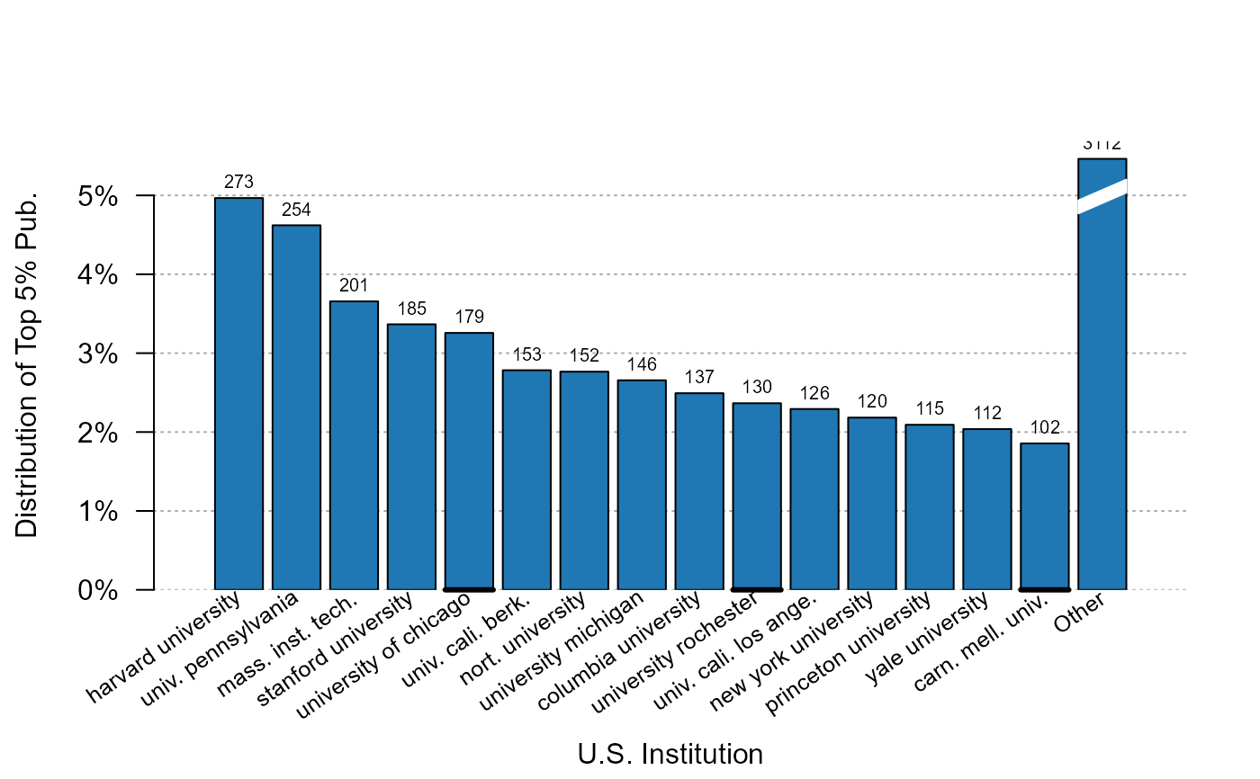
plot_distr(jnl_top_5p ~ institution, us_pub_econ)
 # You can plot several variables:
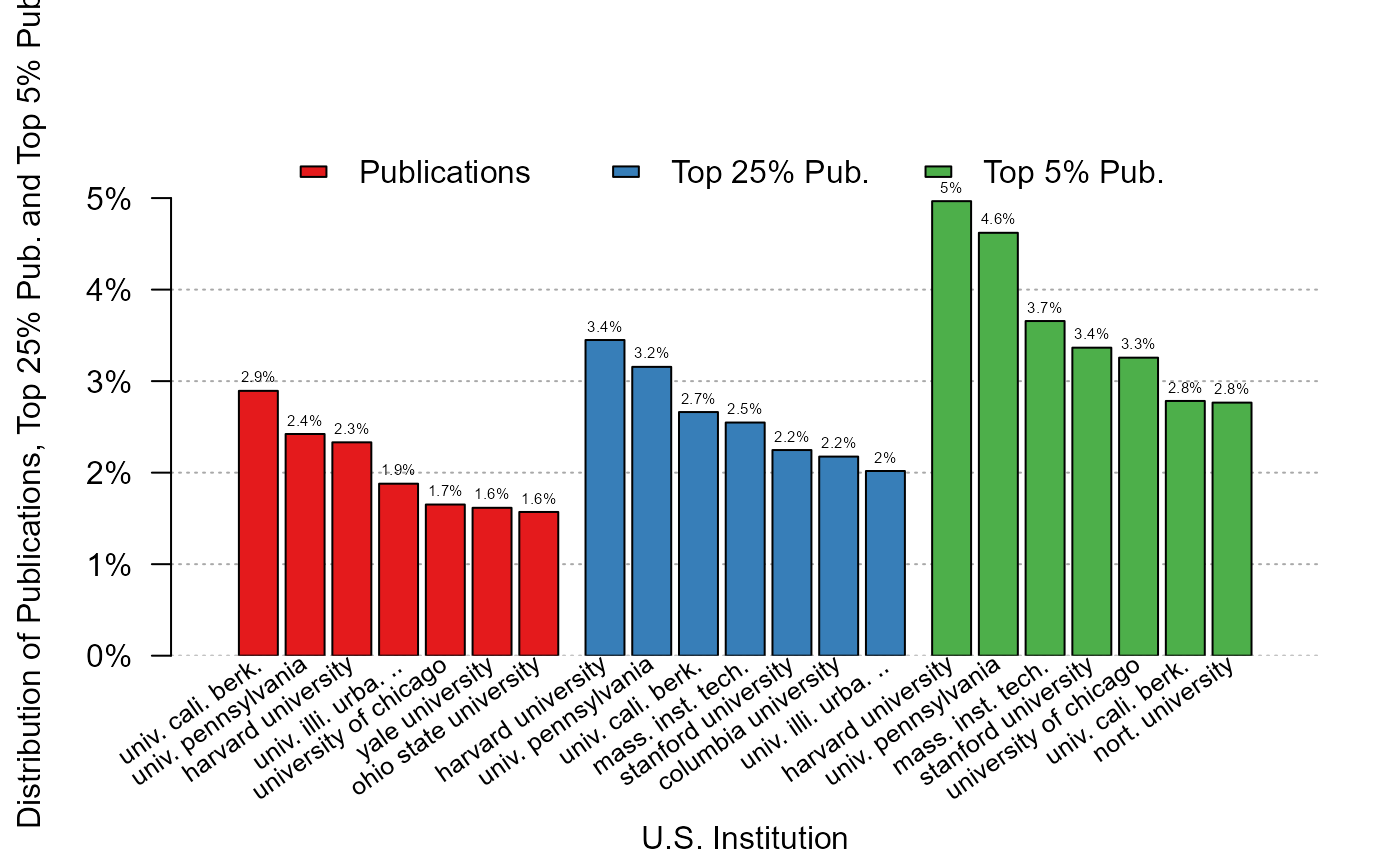
plot_distr(1 + jnl_top_25p + jnl_top_5p ~ institution, us_pub_econ)
 # 3) Let's plot the journal distribution for the top 3 institutions
# We can get the data from the previous graph
graph_data = plot_distr(jnl_top_5p ~ institution, us_pub_econ, plot = FALSE)
# And then select the top universities
top3_instit = graph_data$x[1:3]
top5_instit = graph_data$x[1:5] # we'll use it later
# Now the distribution of journals
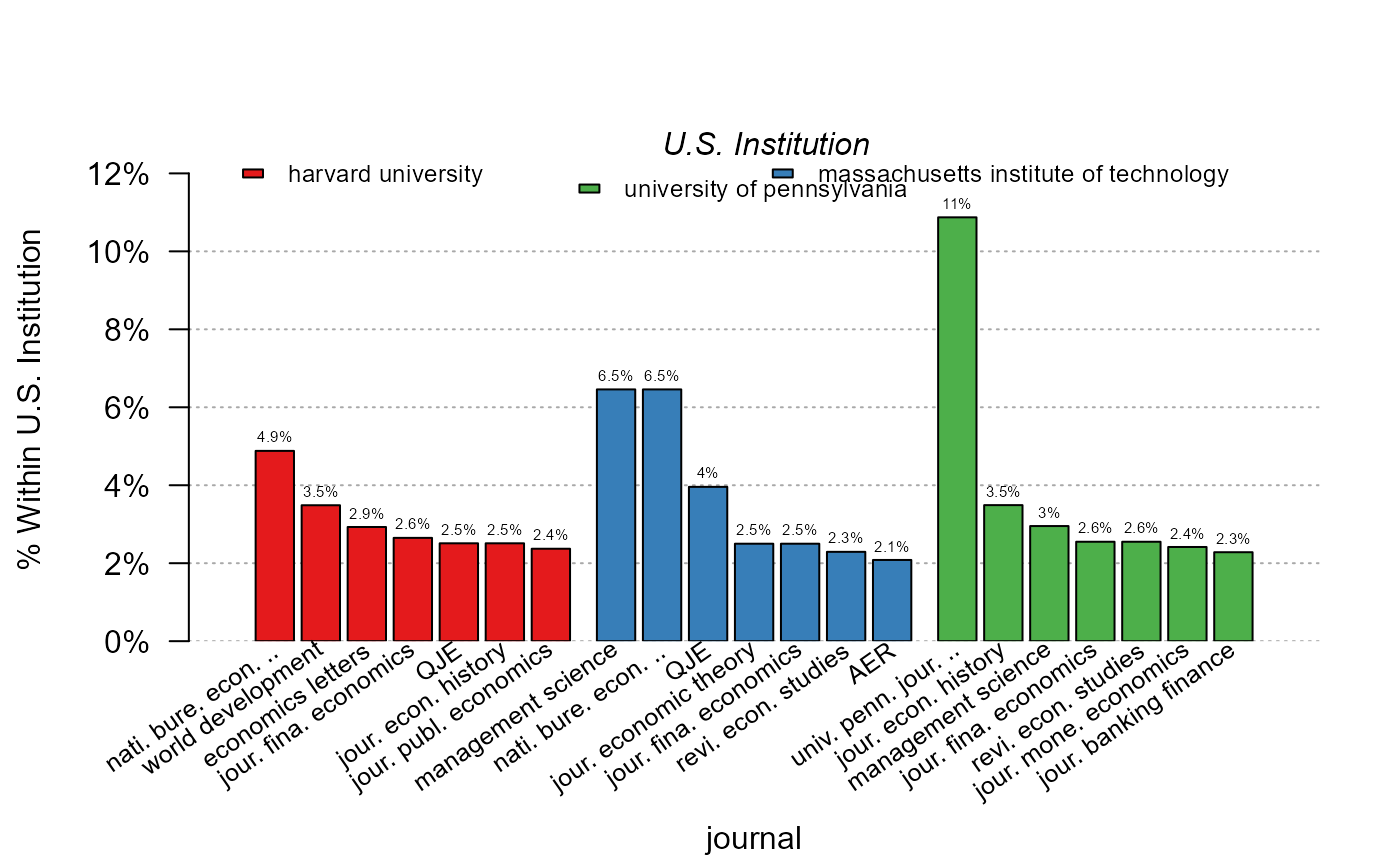
plot_distr(~ journal | institution, us_pub_econ[institution %in% top3_instit])
# Alternatively, you can use the argument mod.select:
plot_distr(~ journal | institution, us_pub_econ, mod.select = top3_instit)
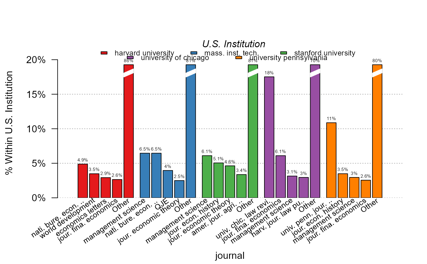
 # 3') Same graph as before with "other" column, 5 institutions
plot_distr(~ journal | institution, us_pub_econ,
mod.select = top5_instit, other = TRUE)
 #
# Example with continuous data
#
# regular histogram
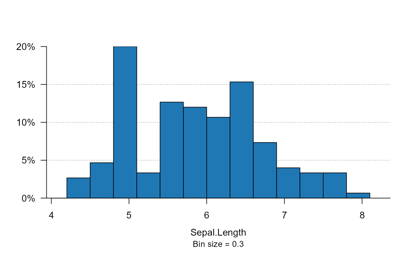
plot_distr(iris$Sepal.Length)
#
# Example with continuous data
#
# regular histogram
plot_distr(iris$Sepal.Length)
 # now splitting by species:
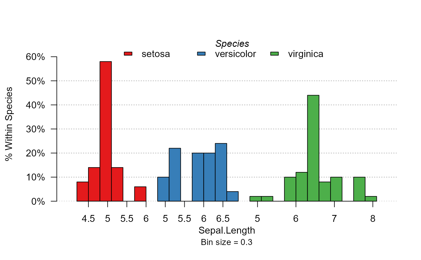
plot_distr(~ Sepal.Length | Species, iris)
 # idem but the three distr. are separated:
plot_distr(~ Sepal.Length | Species, iris, mod.method = "split")
 # Now the three are stacked
plot_distr(~ Sepal.Length | Species, iris, mod.method = "stack")
