Treat a variable as a factor, or interacts a variable with a factor. Values to
be dropped/kept from the factor can be easily set. Note that to interact
fixed-effects, this function should not be used: instead use directly the syntax fe1^fe2.
Arguments
- factor_var
A vector (of any type) that will be treated as a factor. You can set references (i.e. exclude values for which to create dummies) with the
refargument.- var
A variable of the same length as
factor_var. This variable will be interacted with the factor infactor_var. It can be numeric or factor-like. To force a numeric variable to be treated as a factor, you can add thei.prefix to a variable name. For instance take a numeric variablex_num:i(x_fact, x_num)will treatx_numas numeric whilei(x_fact, i.x_num)will treatx_numas a factor (it's a shortcut toas.factor(x_num)).- ref
A vector of values to be taken as references from
factor_var. Can also be a logical: ifTRUE, then the first value offactor_varwill be removed. Ifrefis a character vector, partial matching is applied to values; use "@" as the first character to enable regular expression matching. See examples.- keep
A vector of values to be kept from
factor_var(all others are dropped). By default they should be values fromfactor_varand ifkeepis a character vector partial matching is applied. Use "@" as the first character to enable regular expression matching instead.- bin
A list of values to be grouped, a vector, a formula, or the special values
"bin::digit"or"cut::values". To create a new value from old values, usebin = list("new_value"=old_values)withold_valuesa vector of existing values. You can use.()forlist(). It accepts regular expressions, but they must start with an"@", like inbin="@Aug|Dec". It accepts one-sided formulas which must contain the variablex, e.g.bin=list("<2" = ~x < 2). The names of the list are the new names. If the new name is missing, the first value matched becomes the new name. In the name, adding"@d", withda digit, will relocate the value in positiond: useful to change the position of factors. Use"@"as first item to make subsequent items be located first in the factor. Feeding in a vector is like using a list without name and only a single element. If the vector is numeric, you can use the special value"bin::digit"to group everydigitelement. For example ifxrepresents years, usingbin="bin::2"creates bins of two years. With any data, using"!bin::digit"groups every digit consecutive values starting from the first value. Using"!!bin::digit"is the same but starting from the last value. With numeric vectors you can: a) use"cut::n"to cut the vector intonequal parts, b) use"cut::a]b["to create the following bins:[min, a],]a, b[,[b, max]. The latter syntax is a sequence of number/quartile (q0 to q4)/percentile (p0 to p100) followed by an open or closed square bracket. You can add custom bin names by adding them in the character vector after'cut::values'. See details and examples. Dot square bracket expansion (seedsb) is enabled.- ref2
A vector of values to be dropped from
var. By default they should be values fromvarand ifref2is a character vector partial matching is applied. Use "@" as the first character to enable regular expression matching instead.- keep2
A vector of values to be kept from
var(all others are dropped). By default they should be values fromvarand ifkeep2is a character vector partial matching is applied. Use "@" as the first character to enable regular expression matching instead.- bin2
A list or vector defining the binning of the second variable. See help for the argument
binfor details (or look at the help of the functionbin). You can use.()forlist().- ...
Not currently used.
Value
It returns a matrix with number of rows the length of factor_var. If there is no interacted
variable or it is interacted with a numeric variable, the number of columns is equal to the
number of cases contained in factor_var minus the reference(s). If the interacted variable is
a factor, the number of columns is the number of combined cases between factor_var and var.
Details
To interact fixed-effects, this function should not be used: instead use directly the syntax
fe1^fe2 in the fixed-effects part of the formula. Please see the details and
examples in the help page of feols.
Examples
#
# Simple illustration
#
x = rep(letters[1:4], 3)[1:10]
y = rep(1:4, c(1, 2, 3, 4))
# interaction
data.frame(x, y, i(x, y, ref = TRUE))
#> x y b c d
#> 1 a 1 0 0 0
#> 2 b 2 2 0 0
#> 3 c 2 0 2 0
#> 4 d 3 0 0 3
#> 5 a 3 0 0 0
#> 6 b 3 3 0 0
#> 7 c 4 0 4 0
#> 8 d 4 0 0 4
#> 9 a 4 0 0 0
#> 10 b 4 4 0 0
# without interaction
data.frame(x, i(x, "b"))
#> x a c d
#> 1 a 1 0 0
#> 2 b 0 0 0
#> 3 c 0 1 0
#> 4 d 0 0 1
#> 5 a 1 0 0
#> 6 b 0 0 0
#> 7 c 0 1 0
#> 8 d 0 0 1
#> 9 a 1 0 0
#> 10 b 0 0 0
# you can interact factors too
z = rep(c("e", "f", "g"), c(5, 3, 2))
data.frame(x, z, i(x, z))
#> x z a.e a.g b.e b.f b.g c.e c.f d.e d.f
#> 1 a e 1 0 0 0 0 0 0 0 0
#> 2 b e 0 0 1 0 0 0 0 0 0
#> 3 c e 0 0 0 0 0 1 0 0 0
#> 4 d e 0 0 0 0 0 0 0 1 0
#> 5 a e 1 0 0 0 0 0 0 0 0
#> 6 b f 0 0 0 1 0 0 0 0 0
#> 7 c f 0 0 0 0 0 0 1 0 0
#> 8 d f 0 0 0 0 0 0 0 0 1
#> 9 a g 0 1 0 0 0 0 0 0 0
#> 10 b g 0 0 0 0 1 0 0 0 0
# to force a numeric variable to be treated as a factor: use i.
data.frame(x, y, i(x, i.y))
#> x y a.1 a.3 a.4 b.2 b.3 b.4 c.2 c.4 d.3 d.4
#> 1 a 1 1 0 0 0 0 0 0 0 0 0
#> 2 b 2 0 0 0 1 0 0 0 0 0 0
#> 3 c 2 0 0 0 0 0 0 1 0 0 0
#> 4 d 3 0 0 0 0 0 0 0 0 1 0
#> 5 a 3 0 1 0 0 0 0 0 0 0 0
#> 6 b 3 0 0 0 0 1 0 0 0 0 0
#> 7 c 4 0 0 0 0 0 0 0 1 0 0
#> 8 d 4 0 0 0 0 0 0 0 0 0 1
#> 9 a 4 0 0 1 0 0 0 0 0 0 0
#> 10 b 4 0 0 0 0 0 1 0 0 0 0
# Binning
data.frame(x, i(x, bin = list(ab = c("a", "b"))))
#> x ab c d
#> 1 a 1 0 0
#> 2 b 1 0 0
#> 3 c 0 1 0
#> 4 d 0 0 1
#> 5 a 1 0 0
#> 6 b 1 0 0
#> 7 c 0 1 0
#> 8 d 0 0 1
#> 9 a 1 0 0
#> 10 b 1 0 0
# Same as before but using .() for list() and a regular expression
# note that to trigger a regex, you need to use an @ first
data.frame(x, i(x, bin = .(ab = "@a|b")))
#> x ab c d
#> 1 a 1 0 0
#> 2 b 1 0 0
#> 3 c 0 1 0
#> 4 d 0 0 1
#> 5 a 1 0 0
#> 6 b 1 0 0
#> 7 c 0 1 0
#> 8 d 0 0 1
#> 9 a 1 0 0
#> 10 b 1 0 0
#
# In fixest estimations
#
data(base_did)
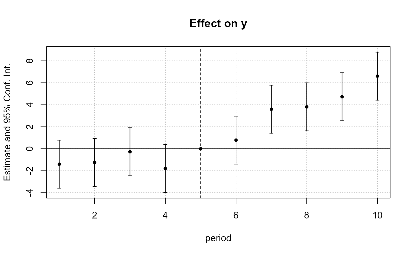
# We interact the variable 'period' with the variable 'treat'
est_did = feols(y ~ x1 + i(period, treat, 5) | id + period, base_did)
# => plot only interactions with iplot
iplot(est_did)
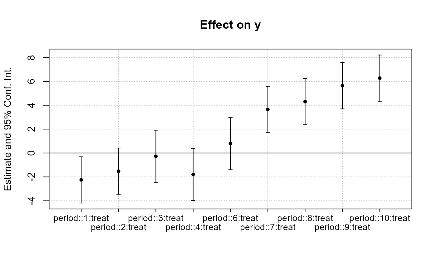
 # Using i() for factors
est_bis = feols(y ~ x1 + i(period, keep = 3:6) + i(period, treat, 5) | id, base_did)
# we plot the second set of variables created with i()
# => we need to use keep (otherwise only the first one is represented)
coefplot(est_bis, keep = "trea")
# Using i() for factors
est_bis = feols(y ~ x1 + i(period, keep = 3:6) + i(period, treat, 5) | id, base_did)
# we plot the second set of variables created with i()
# => we need to use keep (otherwise only the first one is represented)
coefplot(est_bis, keep = "trea")
 # => special treatment in etable
etable(est_bis, dict = c("6" = "six"))
#> est_bis
#> Dependent Var.: y
#>
#> x1 0.9720*** (0.0448)
#> period = 3 -1.111. (0.6064)
#> period = 4 0.4034 (0.6066)
#> period = 5 -0.8980 (0.6066)
#> period = six 0.8031 (0.6064)
#> treat x period = 1 -2.252* (0.9875)
#> treat x period = 2 -1.523 (0.9875)
#> treat x period = 3 -0.2720 (1.113)
#> treat x period = 4 -1.794 (1.113)
#> treat x period = six 0.7850 (1.113)
#> treat x period = 7 3.650*** (0.9875)
#> treat x period = 8 4.310*** (0.9874)
#> treat x period = 9 5.636*** (0.9874)
#> treat x period = 10 6.276*** (0.9875)
#> Fixed-Effects: ------------------
#> id Yes
#> ____________________ __________________
#> S.E. type IID
#> Observations 1,080
#> R2 0.54466
#> Within R2 0.45396
#> ---
#> Signif. codes: 0 '***' 0.001 '**' 0.01 '*' 0.05 '.' 0.1 ' ' 1
#
# Interact two factors
#
# We use the i. prefix to consider week as a factor
data(airquality)
aq = airquality
aq$week = aq$Day %/% 7 + 1
# Interacting Month and week:
res_2F = feols(Ozone ~ Solar.R + i(Month, i.week), aq)
#> NOTE: 42 observations removed because of NA values (LHS: 37, RHS: 7).
# Same but dropping the 5th Month and 1st week
res_2F_bis = feols(Ozone ~ Solar.R + i(Month, i.week, ref = 5, ref2 = 1), aq)
#> NOTE: 42 observations removed because of NA values (LHS: 37, RHS: 7).
etable(res_2F, res_2F_bis)
#> res_2F res_2F_bis
#> Dependent Var.: Ozone Ozone
#>
#> Constant 8.207 (14.16) 18.51* (7.343)
#> Solar.R 0.0963** (0.0314) 0.1007** (0.0324)
#> Month = 5 x week = 2 -11.36 (17.18)
#> Month = 5 x week = 3 -9.660 (16.05)
#> Month = 5 x week = 4 -6.923 (18.28)
#> Month = 5 x week = 5 28.32 (18.10)
#> Month = 6 x week = 2 10.88 (18.13) -0.3936 (14.93)
#> Month = 6 x week = 3 -2.422 (17.22) -13.40 (13.47)
#> Month = 7 x week = 1 31.87. (17.27)
#> Month = 7 x week = 2 34.35* (16.59) 23.00. (12.58)
#> Month = 7 x week = 3 20.17 (16.54) 8.938 (12.47)
#> Month = 7 x week = 4 33.76. (17.26) 22.85. (13.51)
#> Month = 7 x week = 5 31.58. (18.19) 20.19 (15.04)
#> Month = 8 x week = 1 7.218 (19.98)
#> Month = 8 x week = 2 48.12** (17.22) 36.81** (13.56)
#> Month = 8 x week = 3 19.17 (16.62) 8.257 (12.48)
#> Month = 8 x week = 4 36.50* (17.18) 25.35. (13.46)
#> Month = 8 x week = 5 62.00*** (18.12) 50.76*** (14.91)
#> Month = 9 x week = 1 46.47** (16.57)
#> Month = 9 x week = 2 -5.661 (16.12) -17.03 (11.82)
#> Month = 9 x week = 3 -2.978 (16.10) -13.95 (11.65)
#> Month = 9 x week = 4 1.809 (16.73) -8.973 (12.61)
#> Month = 9 x week = 5 -8.373 (19.56) -19.47 (16.95)
#> ____________________ _________________ _________________
#> S.E. type IID IID
#> Observations 111 111
#> R2 0.52636 0.37684
#> Adj. R2 0.40795 0.27844
#> ---
#> Signif. codes: 0 '***' 0.001 '**' 0.01 '*' 0.05 '.' 0.1 ' ' 1
#
# Binning
#
data(airquality)
feols(Ozone ~ i(Month, bin = "bin::2"), airquality)
#> NOTE: 37 observations removed because of NA values (LHS: 37).
#> OLS estimation, Dep. Var.: Ozone
#> Observations: 116
#> Standard-errors: IID
#> Estimate Std. Error t value Pr(>|t|)
#> (Intercept) 23.6154 6.19450 3.81231 0.00022469 ***
#> Month::6 27.8703 8.17782 3.40804 0.00090749 ***
#> Month::8 21.3119 7.51740 2.83501 0.00543040 **
#> ---
#> Signif. codes: 0 '***' 0.001 '**' 0.01 '*' 0.05 '.' 0.1 ' ' 1
#> RMSE: 31.2 Adj. R2: 0.083194
feols(Ozone ~ i(Month, bin = list(summer = 7:9)), airquality)
#> NOTE: 37 observations removed because of NA values (LHS: 37).
#> OLS estimation, Dep. Var.: Ozone
#> Observations: 116
#> Standard-errors: IID
#> Estimate Std. Error t value Pr(>|t|)
#> (Intercept) 23.61538 6.13010 3.852364 0.00019455 ***
#> Month::6 5.82906 12.08872 0.482190 0.63060377
#> Month::summer 25.86610 7.04559 3.671249 0.00037013 ***
#> ---
#> Signif. codes: 0 '***' 0.001 '**' 0.01 '*' 0.05 '.' 0.1 ' ' 1
#> RMSE: 30.9 Adj. R2: 0.102158
# => special treatment in etable
etable(est_bis, dict = c("6" = "six"))
#> est_bis
#> Dependent Var.: y
#>
#> x1 0.9720*** (0.0448)
#> period = 3 -1.111. (0.6064)
#> period = 4 0.4034 (0.6066)
#> period = 5 -0.8980 (0.6066)
#> period = six 0.8031 (0.6064)
#> treat x period = 1 -2.252* (0.9875)
#> treat x period = 2 -1.523 (0.9875)
#> treat x period = 3 -0.2720 (1.113)
#> treat x period = 4 -1.794 (1.113)
#> treat x period = six 0.7850 (1.113)
#> treat x period = 7 3.650*** (0.9875)
#> treat x period = 8 4.310*** (0.9874)
#> treat x period = 9 5.636*** (0.9874)
#> treat x period = 10 6.276*** (0.9875)
#> Fixed-Effects: ------------------
#> id Yes
#> ____________________ __________________
#> S.E. type IID
#> Observations 1,080
#> R2 0.54466
#> Within R2 0.45396
#> ---
#> Signif. codes: 0 '***' 0.001 '**' 0.01 '*' 0.05 '.' 0.1 ' ' 1
#
# Interact two factors
#
# We use the i. prefix to consider week as a factor
data(airquality)
aq = airquality
aq$week = aq$Day %/% 7 + 1
# Interacting Month and week:
res_2F = feols(Ozone ~ Solar.R + i(Month, i.week), aq)
#> NOTE: 42 observations removed because of NA values (LHS: 37, RHS: 7).
# Same but dropping the 5th Month and 1st week
res_2F_bis = feols(Ozone ~ Solar.R + i(Month, i.week, ref = 5, ref2 = 1), aq)
#> NOTE: 42 observations removed because of NA values (LHS: 37, RHS: 7).
etable(res_2F, res_2F_bis)
#> res_2F res_2F_bis
#> Dependent Var.: Ozone Ozone
#>
#> Constant 8.207 (14.16) 18.51* (7.343)
#> Solar.R 0.0963** (0.0314) 0.1007** (0.0324)
#> Month = 5 x week = 2 -11.36 (17.18)
#> Month = 5 x week = 3 -9.660 (16.05)
#> Month = 5 x week = 4 -6.923 (18.28)
#> Month = 5 x week = 5 28.32 (18.10)
#> Month = 6 x week = 2 10.88 (18.13) -0.3936 (14.93)
#> Month = 6 x week = 3 -2.422 (17.22) -13.40 (13.47)
#> Month = 7 x week = 1 31.87. (17.27)
#> Month = 7 x week = 2 34.35* (16.59) 23.00. (12.58)
#> Month = 7 x week = 3 20.17 (16.54) 8.938 (12.47)
#> Month = 7 x week = 4 33.76. (17.26) 22.85. (13.51)
#> Month = 7 x week = 5 31.58. (18.19) 20.19 (15.04)
#> Month = 8 x week = 1 7.218 (19.98)
#> Month = 8 x week = 2 48.12** (17.22) 36.81** (13.56)
#> Month = 8 x week = 3 19.17 (16.62) 8.257 (12.48)
#> Month = 8 x week = 4 36.50* (17.18) 25.35. (13.46)
#> Month = 8 x week = 5 62.00*** (18.12) 50.76*** (14.91)
#> Month = 9 x week = 1 46.47** (16.57)
#> Month = 9 x week = 2 -5.661 (16.12) -17.03 (11.82)
#> Month = 9 x week = 3 -2.978 (16.10) -13.95 (11.65)
#> Month = 9 x week = 4 1.809 (16.73) -8.973 (12.61)
#> Month = 9 x week = 5 -8.373 (19.56) -19.47 (16.95)
#> ____________________ _________________ _________________
#> S.E. type IID IID
#> Observations 111 111
#> R2 0.52636 0.37684
#> Adj. R2 0.40795 0.27844
#> ---
#> Signif. codes: 0 '***' 0.001 '**' 0.01 '*' 0.05 '.' 0.1 ' ' 1
#
# Binning
#
data(airquality)
feols(Ozone ~ i(Month, bin = "bin::2"), airquality)
#> NOTE: 37 observations removed because of NA values (LHS: 37).
#> OLS estimation, Dep. Var.: Ozone
#> Observations: 116
#> Standard-errors: IID
#> Estimate Std. Error t value Pr(>|t|)
#> (Intercept) 23.6154 6.19450 3.81231 0.00022469 ***
#> Month::6 27.8703 8.17782 3.40804 0.00090749 ***
#> Month::8 21.3119 7.51740 2.83501 0.00543040 **
#> ---
#> Signif. codes: 0 '***' 0.001 '**' 0.01 '*' 0.05 '.' 0.1 ' ' 1
#> RMSE: 31.2 Adj. R2: 0.083194
feols(Ozone ~ i(Month, bin = list(summer = 7:9)), airquality)
#> NOTE: 37 observations removed because of NA values (LHS: 37).
#> OLS estimation, Dep. Var.: Ozone
#> Observations: 116
#> Standard-errors: IID
#> Estimate Std. Error t value Pr(>|t|)
#> (Intercept) 23.61538 6.13010 3.852364 0.00019455 ***
#> Month::6 5.82906 12.08872 0.482190 0.63060377
#> Month::summer 25.86610 7.04559 3.671249 0.00037013 ***
#> ---
#> Signif. codes: 0 '***' 0.001 '**' 0.01 '*' 0.05 '.' 0.1 ' ' 1
#> RMSE: 30.9 Adj. R2: 0.102158