You can set formula macros globally with setFixest_fml. These macros can then be used in fixest estimations or when using the function xpd.
Arguments
- ...
Definition of the macro variables. Each argument name corresponds to the name of the macro variable. It is required that each macro variable name starts with two dots (e.g.
..ctrl). The value of each argument must be a one-sided formula or a character vector, it is the definition of the macro variable. Example of a valid call:setFixest_fml(..ctrl = ~ var1 + var2). In the functionxpd, the default macro variables are taken fromgetFixest_fml, any variable in...will replace these values. You can enclose values in.[], if so they will be evaluated from the current environment. For example..ctrl = ~ x.[1:2] + .[z]will lead to~x1 + x2 + varifzis equal to"var".- reset
A logical scalar, defaults to
FALSE. IfTRUE, all macro variables are first reset (i.e. deleted).
Value
The function getFixest_fml() returns a list of character strings, the names
corresponding to the macro variable names, the character strings corresponding
to their definition.
Details
In xpd, the default macro variables are taken from getFixest_fml.
Any value in the ... argument of xpd will replace these default values.
The definitions of the macro variables will replace in verbatim the macro variables.
Therefore, you can include multipart formulas if you wish but then beware of the order the
macros variable in the formula. For example, using the airquality data, say you want to set as
controls the variable Temp and Day fixed-effects, you can do
setFixest_fml(..ctrl = ~Temp | Day), but then
feols(Ozone ~ Wind + ..ctrl, airquality) will be quite different from
feols(Ozone ~ ..ctrl + Wind, airquality), so beware!
See also
xpd to make use of formula macros.
Examples
# Small examples with airquality data
data(airquality)
# we set two macro variables
setFixest_fml(..ctrl = ~ Temp + Day,
..ctrl_long = ~ poly(Temp, 2) + poly(Day, 2))
# Using the macro in lm with xpd:
lm(xpd(Ozone ~ Wind + ..ctrl), airquality)
#>
#> Call:
#> lm(formula = xpd(Ozone ~ Wind + ..ctrl), data = airquality)
#>
#> Coefficients:
#> (Intercept) Wind Temp Day
#> -76.5168 -3.0681 1.8622 0.2506
#>
lm(xpd(Ozone ~ Wind + ..ctrl_long), airquality)
#>
#> Call:
#> lm(formula = xpd(Ozone ~ Wind + ..ctrl_long), data = airquality)
#>
#> Coefficients:
#> (Intercept) Wind poly(Temp, 2)1 poly(Temp, 2)2 poly(Day, 2)1
#> 69.603 -2.773 206.921 90.449 26.681
#> poly(Day, 2)2
#> 20.483
#>
# You can use the macros without xpd() in fixest estimations
a = feols(Ozone ~ Wind + ..ctrl, airquality)
#> NOTE: 37 observations removed because of NA values (LHS: 37).
b = feols(Ozone ~ Wind + ..ctrl_long, airquality)
#> NOTE: 37 observations removed because of NA values (LHS: 37).
etable(a, b, keep = "Int|Win")
#> a b
#> Dependent Var.: Ozone Ozone
#>
#> Wind -3.068*** (0.6629) -2.773*** (0.6451)
#> _______________ __________________ __________________
#> S.E. type IID IID
#> Observations 116 116
#> R2 0.57308 0.62167
#> Adj. R2 0.56164 0.60447
#> ---
#> Signif. codes: 0 '***' 0.001 '**' 0.01 '*' 0.05 '.' 0.1 ' ' 1
# Using .[]
base = setNames(iris, c("y", "x1", "x2", "x3", "species"))
i = 2:3
z = "species"
lm(xpd(y ~ x.[2:3] + .[z]), base)
#>
#> Call:
#> lm(formula = xpd(y ~ x.[2:3] + .[z]), data = base)
#>
#> Coefficients:
#> (Intercept) x2 x3 speciesversicolor
#> 3.682982 0.905946 -0.005995 -1.598362
#> speciesvirginica
#> -2.112647
#>
# No xpd() needed in feols
feols(y ~ x.[2:3] + .[z], base)
#> OLS estimation, Dep. Var.: y
#> Observations: 150
#> Standard-errors: IID
#> Estimate Std. Error t value Pr(>|t|)
#> (Intercept) 3.682982 0.107403 34.291343 < 2.2e-16 ***
#> x2 0.905946 0.074311 12.191282 < 2.2e-16 ***
#> x3 -0.005995 0.156260 -0.038368 9.6945e-01
#> speciesversicolor -1.598362 0.205706 -7.770113 1.3154e-12 ***
#> speciesvirginica -2.112647 0.304024 -6.948940 1.1550e-10 ***
#> ---
#> Signif. codes: 0 '***' 0.001 '**' 0.01 '*' 0.05 '.' 0.1 ' ' 1
#> RMSE: 0.333482 Adj. R2: 0.832221
#
# Auto completion with '..' suffix
#
# You can trigger variables autocompletion with the '..' suffix
# You need to provide the argument data
base = setNames(iris, c("y", "x1", "x2", "x3", "species"))
xpd(y ~ x.., data = base)
#> y ~ x1 + x2 + x3
#> <environment: 0x000001f81833def8>
# In fixest estimations, this is automatically taken care of
feols(y ~ x.., data = base)
#> OLS estimation, Dep. Var.: y
#> Observations: 150
#> Standard-errors: IID
#> Estimate Std. Error t value Pr(>|t|)
#> (Intercept) 1.855997 0.250777 7.40098 9.8539e-12 ***
#> x1 0.650837 0.066647 9.76538 < 2.2e-16 ***
#> x2 0.709132 0.056719 12.50248 < 2.2e-16 ***
#> x3 -0.556483 0.127548 -4.36293 2.4129e-05 ***
#> ---
#> Signif. codes: 0 '***' 0.001 '**' 0.01 '*' 0.05 '.' 0.1 ' ' 1
#> RMSE: 0.310327 Adj. R2: 0.855706
#
# You can use xpd for stepwise estimations
#
# Note that for stepwise estimations in fixest, you can use
# the stepwise functions: sw, sw0, csw, csw0
# -> see help in feols or in the dedicated vignette
# we want to look at the effect of x1 on y
# controlling for different variables
base = iris
names(base) = c("y", "x1", "x2", "x3", "species")
# We first create a matrix with all possible combinations of variables
my_args = lapply(names(base)[-(1:2)], function(x) c("", x))
(all_combs = as.matrix(do.call("expand.grid", my_args)))
#> Var1 Var2 Var3
#> [1,] "" "" ""
#> [2,] "x2" "" ""
#> [3,] "" "x3" ""
#> [4,] "x2" "x3" ""
#> [5,] "" "" "species"
#> [6,] "x2" "" "species"
#> [7,] "" "x3" "species"
#> [8,] "x2" "x3" "species"
res_all = list()
for(i in 1:nrow(all_combs)){
res_all[[i]] = feols(xpd(y ~ x1 + ..v, ..v = all_combs[i, ]), base)
}
etable(res_all)
#> model 1 model 2 model 3
#> Dependent Var.: y y y
#>
#> Constant 6.526*** (0.4789) 2.249*** (0.2480) 3.457*** (0.3092)
#> x1 -0.2234 (0.1551) 0.5955*** (0.0693) 0.3991*** (0.0911)
#> x2 0.4719*** (0.0171)
#> x3 0.9721*** (0.0521)
#> speciesversicolor
#> speciesvirginica
#> _________________ _________________ __________________ __________________
#> S.E. type IID IID IID
#> Observations 150 150 150
#> R2 0.01382 0.84018 0.70724
#> Adj. R2 0.00716 0.83800 0.70325
#>
#> model 4 model 5 model 6
#> Dependent Var.: y y y
#>
#> Constant 1.856*** (0.2508) 2.251*** (0.3698) 2.390*** (0.2623)
#> x1 0.6508*** (0.0667) 0.8036*** (0.1063) 0.4322*** (0.0814)
#> x2 0.7091*** (0.0567) 0.7756*** (0.0643)
#> x3 -0.5565*** (0.1275)
#> speciesversicolor 1.459*** (0.1121) -0.9558*** (0.2152)
#> speciesvirginica 1.947*** (0.1000) -1.394*** (0.2857)
#> _________________ ___________________ __________________ ___________________
#> S.E. type IID IID IID
#> Observations 150 150 150
#> R2 0.85861 0.72591 0.86331
#> Adj. R2 0.85571 0.72027 0.85954
#>
#> model 7 model 8
#> Dependent Var.: y y
#>
#> Constant 2.521*** (0.3939) 2.171*** (0.2798)
#> x1 0.6982*** (0.1195) 0.4959*** (0.0861)
#> x2 0.8292*** (0.0685)
#> x3 0.3716. (0.1983) -0.3152* (0.1512)
#> speciesversicolor 0.9881*** (0.2747) -0.7236** (0.2402)
#> speciesvirginica 1.238** (0.3913) -1.023** (0.3337)
#> _________________ __________________ __________________
#> S.E. type IID IID
#> Observations 150 150
#> R2 0.73238 0.86731
#> Adj. R2 0.72500 0.86271
#> ---
#> Signif. codes: 0 '***' 0.001 '**' 0.01 '*' 0.05 '.' 0.1 ' ' 1
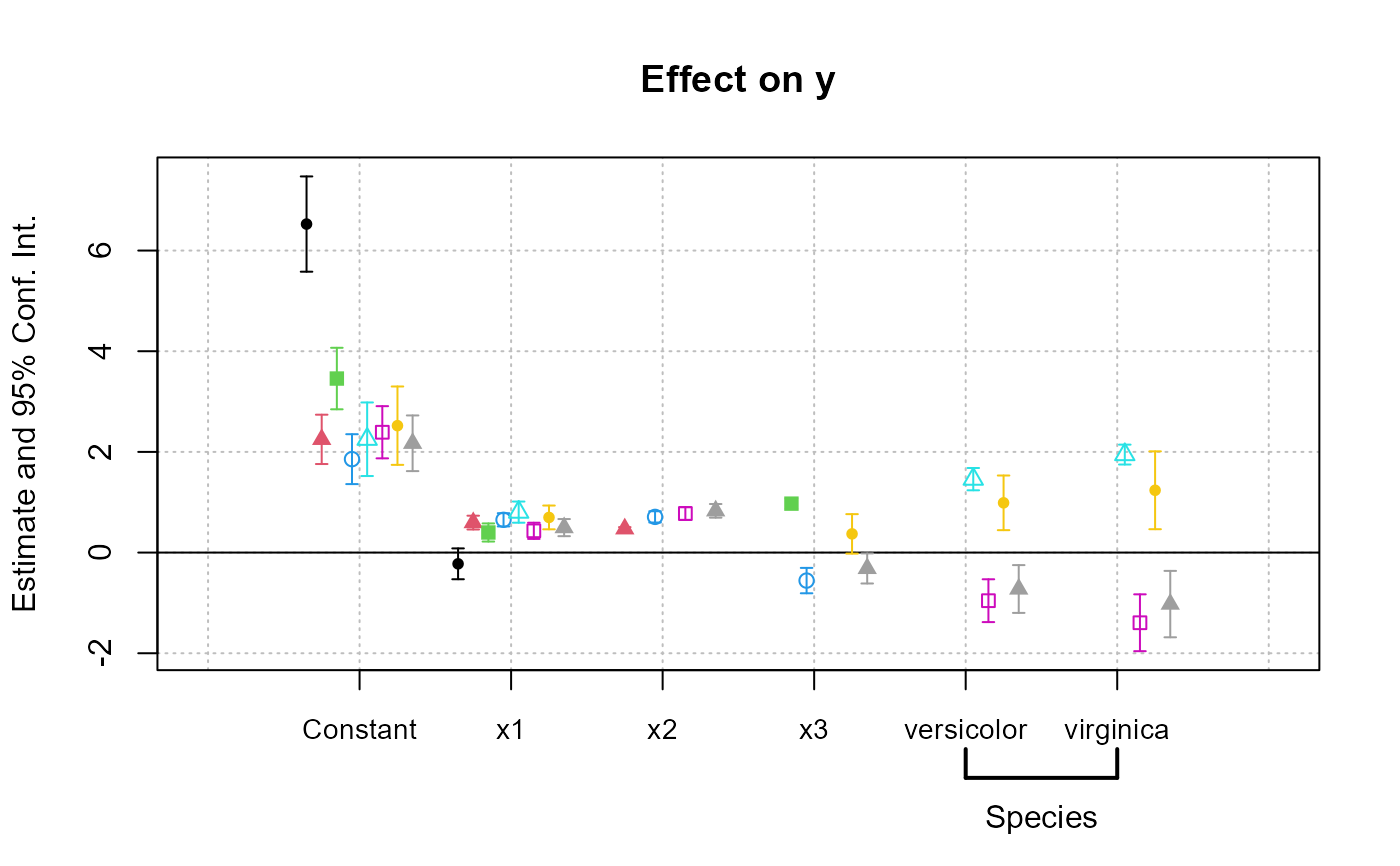
coefplot(res_all, group = list(Species = "^^species"))
 #
# You can use macros to grep variables in your data set
#
# Example 1: setting a macro variable globally
data(longley)
setFixest_fml(..many_vars = grep("GNP|ployed", names(longley), value = TRUE))
feols(Armed.Forces ~ Population + ..many_vars, longley)
#> OLS estimation, Dep. Var.: Armed.Forces
#> Observations: 16
#> Standard-errors: IID
#> Estimate Std. Error t value Pr(>|t|)
#> (Intercept) 4403.682352 4091.847594 1.076209 0.307112
#> Population -22.844324 32.671302 -0.699217 0.500356
#> GNP.deflator 7.638472 12.347773 0.618611 0.550003
#> GNP 3.150533 3.554170 0.886433 0.396201
#> Unemployed -0.591649 0.389005 -1.520928 0.159248
#> Employed -50.059800 25.348299 -1.974878 0.076522 .
#> ---
#> Signif. codes: 0 '***' 0.001 '**' 0.01 '*' 0.05 '.' 0.1 ' ' 1
#> RMSE: 36.1 Adj. R2: 0.569345
# Example 2: using ..("regex") or regex("regex") to grep the variables "live"
feols(Armed.Forces ~ Population + ..("GNP|ployed"), longley)
#> OLS estimation, Dep. Var.: Armed.Forces
#> Observations: 16
#> Standard-errors: IID
#> Estimate Std. Error t value Pr(>|t|)
#> (Intercept) 4403.682352 4091.847594 1.076209 0.307112
#> Population -22.844324 32.671302 -0.699217 0.500356
#> GNP.deflator 7.638472 12.347773 0.618611 0.550003
#> GNP 3.150533 3.554170 0.886433 0.396201
#> Unemployed -0.591649 0.389005 -1.520928 0.159248
#> Employed -50.059800 25.348299 -1.974878 0.076522 .
#> ---
#> Signif. codes: 0 '***' 0.001 '**' 0.01 '*' 0.05 '.' 0.1 ' ' 1
#> RMSE: 36.1 Adj. R2: 0.569345
# Example 3: same as Ex.2 but without using a fixest estimation
# Here we need to use xpd():
lm(xpd(Armed.Forces ~ Population + regex("GNP|ployed"), data = longley), longley)
#>
#> Call:
#> lm(formula = xpd(Armed.Forces ~ Population + regex("GNP|ployed"),
#> data = longley), data = longley)
#>
#> Coefficients:
#> (Intercept) Population GNP.deflator GNP Unemployed
#> 4403.6824 -22.8443 7.6385 3.1505 -0.5916
#> Employed
#> -50.0598
#>
# Stepwise estimation with regex: use a comma after the parenthesis
feols(Armed.Forces ~ Population + sw(regex(,"GNP|ployed")), longley)
#> x.1 x.2 x.3
#> Dependent Var.: Armed.Forces Armed.Forces Armed.Forces
#>
#> Constant 1,126.8. (573.7) 4,123.9** (1,276.6) -627.5* (282.9)
#> Population -21.99. (10.45) -44.01** (14.09) 9.202** (2.755)
#> GNP.deflator 16.88* (6.735)
#> GNP 3.365** (0.9860)
#> Unemployed -0.6024* (0.2051)
#> Employed
#> _______________ ________________ ___________________ _________________
#> S.E. type IID IID IID
#> Observations 16 16 16
#> R2 0.41523 0.54263 0.47868
#> Adj. R2 0.32526 0.47226 0.39848
#>
#> x.4
#> Dependent Var.: Armed.Forces
#>
#> Constant -397.0 (310.2)
#> Population -9.634 (8.443)
#> GNP.deflator
#> GNP
#> Unemployed
#> Employed 27.39 (16.72)
#> _______________ ______________
#> S.E. type IID
#> Observations 16
#> R2 0.28114
#> Adj. R2 0.17055
#> ---
#> Signif. codes: 0 '***' 0.001 '**' 0.01 '*' 0.05 '.' 0.1 ' ' 1
# Multiple LHS
etable(feols(..("GNP|ployed") ~ Population, longley))
#> feols(..("GNP|..1 feols(..("GNP|pl..2 feols(..("GN..3
#> Dependent Var.: GNP.deflator GNP Unemployed
#>
#> Constant -76.69*** (9.903) -1,275.2*** (59.83) -763.7* (307.0)
#> Population 1.519*** (0.0842) 14.16*** (0.5086) 9.223** (2.610)
#> _______________ _________________ ___________________ _______________
#> S.E. type IID IID IID
#> Observations 16 16 16
#> R2 0.95876 0.98226 0.47135
#> Adj. R2 0.95582 0.98099 0.43359
#>
#> feols(..("GNP|p..4
#> Dependent Var.: Employed
#>
#> Constant 8.381. (4.422)
#> Population 0.4849*** (0.0376)
#> _______________ __________________
#> S.E. type IID
#> Observations 16
#> R2 0.92235
#> Adj. R2 0.91680
#> ---
#> Signif. codes: 0 '***' 0.001 '**' 0.01 '*' 0.05 '.' 0.1 ' ' 1
#
# lhs and rhs arguments
#
# to create a one sided formula from a character vector
vars = letters[1:5]
xpd(rhs = vars)
#> ~a + b + c + d + e
#> <environment: 0x000001f81833def8>
# Alternatively, to replace the RHS
xpd(y ~ 1, rhs = vars)
#> y ~ a + b + c + d + e
#> <environment: 0x000001f81833def8>
# To create a two sided formula
xpd(lhs = "y", rhs = vars)
#> y ~ a + b + c + d + e
#> <environment: 0x000001f81833def8>
#
# argument 'add'
#
xpd(~x1, add = ~ x2 + x3)
#> ~x1 + x2 + x3
#> <environment: 0x000001f81833def8>
# also works with character vectors
xpd(~x1, add = c("x2", "x3"))
#> ~x1 + x2 + x3
#> <environment: 0x000001f81833def8>
# only adds to the RHS
xpd(y ~ x, add = ~bon + jour)
#> y ~ x + bon + jour
#> <environment: 0x000001f81833def8>
#
# argument add.after_pipe
#
xpd(~x1, add.after_pipe = ~ x2 + x3)
#> ~x1 | x2 + x3
#> <environment: 0x000001f81833def8>
# we can add a two sided formula
xpd(~x1, add.after_pipe = x2 ~ x3)
#> ~x1 | x2 ~ x3
#> <environment: 0x000001f81833def8>
#
# Dot square bracket operator
#
# The basic use is to add variables in the formula
x = c("x1", "x2")
xpd(y ~ .[x])
#> y ~ x1 + x2
#> <environment: 0x000001f81833def8>
# Alternatively, one-sided formulas can be used and their content will be inserted verbatim
x = ~x1 + x2
xpd(y ~ .[x])
#> y ~ x1 + x2
#> <environment: 0x000001f81833def8>
# You can create multiple variables at once
xpd(y ~ x.[1:5] + z.[2:3])
#> y ~ x1 + x2 + x3 + x4 + x5 + z2 + z3
#> <environment: 0x000001f81833def8>
# You can summon variables from the environment to complete variables names
var = "a"
xpd(y ~ x.[var])
#> y ~ xa
#> <environment: 0x000001f81833def8>
# ... the variables can be multiple
vars = LETTERS[1:3]
xpd(y ~ x.[vars])
#> y ~ xA + xB + xC
#> <environment: 0x000001f81833def8>
# You can have "complex" variable names but they must be nested in character form
xpd(y ~ .["x.[vars]_sq"])
#> y ~ xA_sq + xB_sq + xC_sq
#> <environment: 0x000001f81833def8>
# DSB can be used within regular expressions
re = c("GNP", "Pop")
xpd(Unemployed ~ regex(".[re]"), data = longley)
#> Unemployed ~ GNP.deflator + GNP + Population
#> <environment: 0x000001f81833def8>
# => equivalent to regex("GNP|Pop")
# Use .[,var] (NOTE THE COMMA!) to expand with commas
# !! can break the formula if missused
vars = c("wage", "unemp")
xpd(c(y.[,1:3]) ~ csw(.[,vars]))
#> c(y1, y2, y3) ~ csw(wage, unemp)
#> <environment: 0x000001f81833def8>
# Example of use of .[] within a loop
res_all = list()
for(p in 1:3){
res_all[[p]] = feols(Ozone ~ Wind + poly(Temp, .[p]), airquality)
}
#> NOTE: 37 observations removed because of NA values (LHS: 37).
#> NOTE: 37 observations removed because of NA values (LHS: 37).
#> NOTE: 37 observations removed because of NA values (LHS: 37).
etable(res_all)
#> model 1 model 2 model 3
#> Dependent Var.: Ozone Ozone Ozone
#>
#> Constant 72.28*** (6.847) 70.40*** (6.518) 71.31*** (6.512)
#> Wind -3.055*** (0.6633) -2.866*** (0.6315) -2.928*** (0.6295)
#> poly(Temp, 1) 214.7*** (29.17)
#> poly(Temp, 2)1 209.0*** (27.73)
#> poly(Temp, 2)2 93.36*** (25.44)
#> poly(Temp, 3)1 201.5*** (28.02)
#> poly(Temp, 3)2 101.7*** (25.91)
#> poly(Temp, 3)3 -37.32 (25.03)
#> _______________ __________________ __________________ __________________
#> S.E. type IID IID IID
#> Observations 116 116 116
#> R2 0.56871 0.61501 0.62256
#> Adj. R2 0.56108 0.60469 0.60896
#> ---
#> Signif. codes: 0 '***' 0.001 '**' 0.01 '*' 0.05 '.' 0.1 ' ' 1
# The former can be compactly estimated with:
res_compact = feols(Ozone ~ Wind + sw(.[, "poly(Temp, .[1:3])"]), airquality)
#> NOTE: 37 observations removed because of NA values (LHS: 37).
#> |-> this msg only concerns the variables common to all estimations
etable(res_compact)
#> res_compact.1 res_compact.2 res_compact.3
#> Dependent Var.: Ozone Ozone Ozone
#>
#> Constant 72.28*** (6.847) 70.40*** (6.518) 71.31*** (6.512)
#> Wind -3.055*** (0.6633) -2.866*** (0.6315) -2.928*** (0.6295)
#> poly(Temp, 1) 214.7*** (29.17)
#> poly(Temp, 2)1 209.0*** (27.73)
#> poly(Temp, 2)2 93.36*** (25.44)
#> poly(Temp, 3)1 201.5*** (28.02)
#> poly(Temp, 3)2 101.7*** (25.91)
#> poly(Temp, 3)3 -37.32 (25.03)
#> _______________ __________________ __________________ __________________
#> S.E. type IID IID IID
#> Observations 116 116 116
#> R2 0.56871 0.61501 0.62256
#> Adj. R2 0.56108 0.60469 0.60896
#> ---
#> Signif. codes: 0 '***' 0.001 '**' 0.01 '*' 0.05 '.' 0.1 ' ' 1
# How does it work?
# 1) .[, stuff] evaluates stuff and, if a vector, aggregates it with commas
# Comma aggregation is done thanks to the comma placed after the square bracket
# If .[stuff], then aggregation is with sums.
# 2) stuff is evaluated, and if it is a character string, it is evaluated with
# the function dsb which expands values in .[]
#
# Wrapping up:
# 2) evaluation of dsb("poly(Temp, .[1:3])") leads to the vector:
# c("poly(Temp, 1)", "poly(Temp, 2)", "poly(Temp, 3)")
# 1) .[, c("poly(Temp, 1)", "poly(Temp, 2)", "poly(Temp, 3)")] leads to
# poly(Temp, 1), poly(Temp, 2), poly(Temp, 3)
#
# Hence sw(.[, "poly(Temp, .[1:3])"]) becomes:
# sw(poly(Temp, 1), poly(Temp, 2), poly(Temp, 3))
#
# In non-fixest functions: guessing the data allows to use regex
#
# When used in non-fixest functions, the algorithm tries to "guess" the data
# so that ..("regex") can be directly evaluated without passing the argument 'data'
data(longley)
lm(xpd(Armed.Forces ~ Population + ..("GNP|ployed")), longley)
#>
#> Call:
#> lm(formula = xpd(Armed.Forces ~ Population + ..("GNP|ployed")),
#> data = longley)
#>
#> Coefficients:
#> (Intercept) Population GNP.deflator GNP Unemployed
#> 4403.6824 -22.8443 7.6385 3.1505 -0.5916
#> Employed
#> -50.0598
#>
# same for the auto completion with '..'
lm(xpd(Armed.Forces ~ Population + GN..), longley)
#>
#> Call:
#> lm(formula = xpd(Armed.Forces ~ Population + GN..), data = longley)
#>
#> Coefficients:
#> (Intercept) Population GNP.deflator GNP
#> 3901.079 -43.219 2.522 3.039
#>
#
# You can use macros to grep variables in your data set
#
# Example 1: setting a macro variable globally
data(longley)
setFixest_fml(..many_vars = grep("GNP|ployed", names(longley), value = TRUE))
feols(Armed.Forces ~ Population + ..many_vars, longley)
#> OLS estimation, Dep. Var.: Armed.Forces
#> Observations: 16
#> Standard-errors: IID
#> Estimate Std. Error t value Pr(>|t|)
#> (Intercept) 4403.682352 4091.847594 1.076209 0.307112
#> Population -22.844324 32.671302 -0.699217 0.500356
#> GNP.deflator 7.638472 12.347773 0.618611 0.550003
#> GNP 3.150533 3.554170 0.886433 0.396201
#> Unemployed -0.591649 0.389005 -1.520928 0.159248
#> Employed -50.059800 25.348299 -1.974878 0.076522 .
#> ---
#> Signif. codes: 0 '***' 0.001 '**' 0.01 '*' 0.05 '.' 0.1 ' ' 1
#> RMSE: 36.1 Adj. R2: 0.569345
# Example 2: using ..("regex") or regex("regex") to grep the variables "live"
feols(Armed.Forces ~ Population + ..("GNP|ployed"), longley)
#> OLS estimation, Dep. Var.: Armed.Forces
#> Observations: 16
#> Standard-errors: IID
#> Estimate Std. Error t value Pr(>|t|)
#> (Intercept) 4403.682352 4091.847594 1.076209 0.307112
#> Population -22.844324 32.671302 -0.699217 0.500356
#> GNP.deflator 7.638472 12.347773 0.618611 0.550003
#> GNP 3.150533 3.554170 0.886433 0.396201
#> Unemployed -0.591649 0.389005 -1.520928 0.159248
#> Employed -50.059800 25.348299 -1.974878 0.076522 .
#> ---
#> Signif. codes: 0 '***' 0.001 '**' 0.01 '*' 0.05 '.' 0.1 ' ' 1
#> RMSE: 36.1 Adj. R2: 0.569345
# Example 3: same as Ex.2 but without using a fixest estimation
# Here we need to use xpd():
lm(xpd(Armed.Forces ~ Population + regex("GNP|ployed"), data = longley), longley)
#>
#> Call:
#> lm(formula = xpd(Armed.Forces ~ Population + regex("GNP|ployed"),
#> data = longley), data = longley)
#>
#> Coefficients:
#> (Intercept) Population GNP.deflator GNP Unemployed
#> 4403.6824 -22.8443 7.6385 3.1505 -0.5916
#> Employed
#> -50.0598
#>
# Stepwise estimation with regex: use a comma after the parenthesis
feols(Armed.Forces ~ Population + sw(regex(,"GNP|ployed")), longley)
#> x.1 x.2 x.3
#> Dependent Var.: Armed.Forces Armed.Forces Armed.Forces
#>
#> Constant 1,126.8. (573.7) 4,123.9** (1,276.6) -627.5* (282.9)
#> Population -21.99. (10.45) -44.01** (14.09) 9.202** (2.755)
#> GNP.deflator 16.88* (6.735)
#> GNP 3.365** (0.9860)
#> Unemployed -0.6024* (0.2051)
#> Employed
#> _______________ ________________ ___________________ _________________
#> S.E. type IID IID IID
#> Observations 16 16 16
#> R2 0.41523 0.54263 0.47868
#> Adj. R2 0.32526 0.47226 0.39848
#>
#> x.4
#> Dependent Var.: Armed.Forces
#>
#> Constant -397.0 (310.2)
#> Population -9.634 (8.443)
#> GNP.deflator
#> GNP
#> Unemployed
#> Employed 27.39 (16.72)
#> _______________ ______________
#> S.E. type IID
#> Observations 16
#> R2 0.28114
#> Adj. R2 0.17055
#> ---
#> Signif. codes: 0 '***' 0.001 '**' 0.01 '*' 0.05 '.' 0.1 ' ' 1
# Multiple LHS
etable(feols(..("GNP|ployed") ~ Population, longley))
#> feols(..("GNP|..1 feols(..("GNP|pl..2 feols(..("GN..3
#> Dependent Var.: GNP.deflator GNP Unemployed
#>
#> Constant -76.69*** (9.903) -1,275.2*** (59.83) -763.7* (307.0)
#> Population 1.519*** (0.0842) 14.16*** (0.5086) 9.223** (2.610)
#> _______________ _________________ ___________________ _______________
#> S.E. type IID IID IID
#> Observations 16 16 16
#> R2 0.95876 0.98226 0.47135
#> Adj. R2 0.95582 0.98099 0.43359
#>
#> feols(..("GNP|p..4
#> Dependent Var.: Employed
#>
#> Constant 8.381. (4.422)
#> Population 0.4849*** (0.0376)
#> _______________ __________________
#> S.E. type IID
#> Observations 16
#> R2 0.92235
#> Adj. R2 0.91680
#> ---
#> Signif. codes: 0 '***' 0.001 '**' 0.01 '*' 0.05 '.' 0.1 ' ' 1
#
# lhs and rhs arguments
#
# to create a one sided formula from a character vector
vars = letters[1:5]
xpd(rhs = vars)
#> ~a + b + c + d + e
#> <environment: 0x000001f81833def8>
# Alternatively, to replace the RHS
xpd(y ~ 1, rhs = vars)
#> y ~ a + b + c + d + e
#> <environment: 0x000001f81833def8>
# To create a two sided formula
xpd(lhs = "y", rhs = vars)
#> y ~ a + b + c + d + e
#> <environment: 0x000001f81833def8>
#
# argument 'add'
#
xpd(~x1, add = ~ x2 + x3)
#> ~x1 + x2 + x3
#> <environment: 0x000001f81833def8>
# also works with character vectors
xpd(~x1, add = c("x2", "x3"))
#> ~x1 + x2 + x3
#> <environment: 0x000001f81833def8>
# only adds to the RHS
xpd(y ~ x, add = ~bon + jour)
#> y ~ x + bon + jour
#> <environment: 0x000001f81833def8>
#
# argument add.after_pipe
#
xpd(~x1, add.after_pipe = ~ x2 + x3)
#> ~x1 | x2 + x3
#> <environment: 0x000001f81833def8>
# we can add a two sided formula
xpd(~x1, add.after_pipe = x2 ~ x3)
#> ~x1 | x2 ~ x3
#> <environment: 0x000001f81833def8>
#
# Dot square bracket operator
#
# The basic use is to add variables in the formula
x = c("x1", "x2")
xpd(y ~ .[x])
#> y ~ x1 + x2
#> <environment: 0x000001f81833def8>
# Alternatively, one-sided formulas can be used and their content will be inserted verbatim
x = ~x1 + x2
xpd(y ~ .[x])
#> y ~ x1 + x2
#> <environment: 0x000001f81833def8>
# You can create multiple variables at once
xpd(y ~ x.[1:5] + z.[2:3])
#> y ~ x1 + x2 + x3 + x4 + x5 + z2 + z3
#> <environment: 0x000001f81833def8>
# You can summon variables from the environment to complete variables names
var = "a"
xpd(y ~ x.[var])
#> y ~ xa
#> <environment: 0x000001f81833def8>
# ... the variables can be multiple
vars = LETTERS[1:3]
xpd(y ~ x.[vars])
#> y ~ xA + xB + xC
#> <environment: 0x000001f81833def8>
# You can have "complex" variable names but they must be nested in character form
xpd(y ~ .["x.[vars]_sq"])
#> y ~ xA_sq + xB_sq + xC_sq
#> <environment: 0x000001f81833def8>
# DSB can be used within regular expressions
re = c("GNP", "Pop")
xpd(Unemployed ~ regex(".[re]"), data = longley)
#> Unemployed ~ GNP.deflator + GNP + Population
#> <environment: 0x000001f81833def8>
# => equivalent to regex("GNP|Pop")
# Use .[,var] (NOTE THE COMMA!) to expand with commas
# !! can break the formula if missused
vars = c("wage", "unemp")
xpd(c(y.[,1:3]) ~ csw(.[,vars]))
#> c(y1, y2, y3) ~ csw(wage, unemp)
#> <environment: 0x000001f81833def8>
# Example of use of .[] within a loop
res_all = list()
for(p in 1:3){
res_all[[p]] = feols(Ozone ~ Wind + poly(Temp, .[p]), airquality)
}
#> NOTE: 37 observations removed because of NA values (LHS: 37).
#> NOTE: 37 observations removed because of NA values (LHS: 37).
#> NOTE: 37 observations removed because of NA values (LHS: 37).
etable(res_all)
#> model 1 model 2 model 3
#> Dependent Var.: Ozone Ozone Ozone
#>
#> Constant 72.28*** (6.847) 70.40*** (6.518) 71.31*** (6.512)
#> Wind -3.055*** (0.6633) -2.866*** (0.6315) -2.928*** (0.6295)
#> poly(Temp, 1) 214.7*** (29.17)
#> poly(Temp, 2)1 209.0*** (27.73)
#> poly(Temp, 2)2 93.36*** (25.44)
#> poly(Temp, 3)1 201.5*** (28.02)
#> poly(Temp, 3)2 101.7*** (25.91)
#> poly(Temp, 3)3 -37.32 (25.03)
#> _______________ __________________ __________________ __________________
#> S.E. type IID IID IID
#> Observations 116 116 116
#> R2 0.56871 0.61501 0.62256
#> Adj. R2 0.56108 0.60469 0.60896
#> ---
#> Signif. codes: 0 '***' 0.001 '**' 0.01 '*' 0.05 '.' 0.1 ' ' 1
# The former can be compactly estimated with:
res_compact = feols(Ozone ~ Wind + sw(.[, "poly(Temp, .[1:3])"]), airquality)
#> NOTE: 37 observations removed because of NA values (LHS: 37).
#> |-> this msg only concerns the variables common to all estimations
etable(res_compact)
#> res_compact.1 res_compact.2 res_compact.3
#> Dependent Var.: Ozone Ozone Ozone
#>
#> Constant 72.28*** (6.847) 70.40*** (6.518) 71.31*** (6.512)
#> Wind -3.055*** (0.6633) -2.866*** (0.6315) -2.928*** (0.6295)
#> poly(Temp, 1) 214.7*** (29.17)
#> poly(Temp, 2)1 209.0*** (27.73)
#> poly(Temp, 2)2 93.36*** (25.44)
#> poly(Temp, 3)1 201.5*** (28.02)
#> poly(Temp, 3)2 101.7*** (25.91)
#> poly(Temp, 3)3 -37.32 (25.03)
#> _______________ __________________ __________________ __________________
#> S.E. type IID IID IID
#> Observations 116 116 116
#> R2 0.56871 0.61501 0.62256
#> Adj. R2 0.56108 0.60469 0.60896
#> ---
#> Signif. codes: 0 '***' 0.001 '**' 0.01 '*' 0.05 '.' 0.1 ' ' 1
# How does it work?
# 1) .[, stuff] evaluates stuff and, if a vector, aggregates it with commas
# Comma aggregation is done thanks to the comma placed after the square bracket
# If .[stuff], then aggregation is with sums.
# 2) stuff is evaluated, and if it is a character string, it is evaluated with
# the function dsb which expands values in .[]
#
# Wrapping up:
# 2) evaluation of dsb("poly(Temp, .[1:3])") leads to the vector:
# c("poly(Temp, 1)", "poly(Temp, 2)", "poly(Temp, 3)")
# 1) .[, c("poly(Temp, 1)", "poly(Temp, 2)", "poly(Temp, 3)")] leads to
# poly(Temp, 1), poly(Temp, 2), poly(Temp, 3)
#
# Hence sw(.[, "poly(Temp, .[1:3])"]) becomes:
# sw(poly(Temp, 1), poly(Temp, 2), poly(Temp, 3))
#
# In non-fixest functions: guessing the data allows to use regex
#
# When used in non-fixest functions, the algorithm tries to "guess" the data
# so that ..("regex") can be directly evaluated without passing the argument 'data'
data(longley)
lm(xpd(Armed.Forces ~ Population + ..("GNP|ployed")), longley)
#>
#> Call:
#> lm(formula = xpd(Armed.Forces ~ Population + ..("GNP|ployed")),
#> data = longley)
#>
#> Coefficients:
#> (Intercept) Population GNP.deflator GNP Unemployed
#> 4403.6824 -22.8443 7.6385 3.1505 -0.5916
#> Employed
#> -50.0598
#>
# same for the auto completion with '..'
lm(xpd(Armed.Forces ~ Population + GN..), longley)
#>
#> Call:
#> lm(formula = xpd(Armed.Forces ~ Population + GN..), data = longley)
#>
#> Coefficients:
#> (Intercept) Population GNP.deflator GNP
#> 3901.079 -43.219 2.522 3.039
#>